Advanced Methods for Linear ODEs

A Guide to Connection Problems, Exact WKB, and Spectral Applications

A linear ODE can be solved locally without revealing how its solutions fit together globally. This guide begins where local existence theory leaves off: with the connection matrices, monodromy, Stokes data, and boundary functions that turn local solutions into spectra and physical response.

Begin with a complete calculation

The primary scope is second-order complex linear ODEs and rank-two systems, with applications in mathematical physics. Choose a first problem before following the longer chapter sequence:

• Find a connection coefficient. Start with an analytic solution of a Gauss equation at one endpoint, determine its behavior at the other, and verify the answer with local series.
• Find a spectrum. Derive the oscillator quantization rule from two decay conditions, identify the turning-point phases, and check an exact boundary Wronskian.

Each starter specifies its prerequisites, a core first-session reading, progressive hints, and an optional numerical extension. The reading instructions explain how to continue through the full analytic foundation or a selected application. The focused study routes give section-level assignments and checkpoints for three common goals.

The organizing connection problem

For canonically normalized fundamental solutions $\Phi_\alpha$ and $\Phi_\beta$ in two regions, the organizing equation is

$$\Phi_\beta(z)=\Phi_\alpha(z)\,C_{\alpha\beta}.$$

The matrix $C_{\alpha\beta}$ is simple to write and often difficult to compute. Its entries can be obtained directly from Wronskians, analytic continuation, recurrences, or numerical matching. In suitable families, selected parts of the same global data can instead be encoded by isomonodromic tau functions, conformal blocks, quantum periods, Seiberg–Witten/Nekrasov–Shatashvili quantities, spectral determinants, ODE/IM functional relations, or TBA equations.

The master problem

Given normalized local or sectorial solutions of a linear ODE, compute their global connection data and extract the spectral or physical consequences.

The guide develops this problem for second-order complex linear ODEs and their locally equivalent traceless rank-two systems. Higher-order equations enter where they are intrinsic to ODE/IM. Global equivalence requires additional geometric information; the qualification below can be read after the first concrete calculation.

Global qualifications for rank-two systems

Three constructions are kept separate: a single-valued trace-zero gauge of a given $GL(2)$ system uses a horizontal determinant trivialization; an $SL(2)$ lift of its projectivization is a lifting or twisting problem; and a scalar oper realization uses a theta characteristic. These are explained in the global conventions.

From local bases to global data

Write a fundamental matrix with columns formed from two independent scalar solutions,

$$\Phi_\alpha(z)= \begin{pmatrix} y_{\alpha,1}(z) & y_{\alpha,2}(z)\\ y'_{\alpha,1}(z) & y'_{\alpha,2}(z) \end{pmatrix}.$$

A connection matrix is meaningful only with specified basis normalizations. If the two bases are changed by constant invertible matrices,

$$\widetilde{\Phi}_\alpha=\Phi_\alpha G_\alpha, \qquad \widetilde{\Phi}_\beta=\Phi_\beta G_\beta,$$

then the same continuation problem is represented by

$$\widetilde C_{\alpha\beta} =G_\alpha^{-1}C_{\alpha\beta}G_\beta.$$

Thus a bare gamma-function formula, continued fraction, tau function, or period is not yet a connection formula. One must also specify the equation, bases, leading normalizations, branches, continuation path, resonant exceptions, and—at an irregular singularity—the sectors and lateral summation prescription.

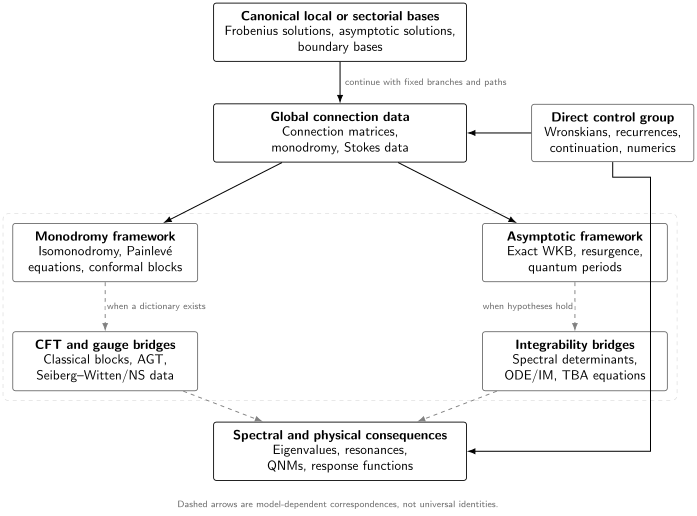
The guide is organized around global connection data. Solid arrows are direct ODE constructions or checks; dashed arrows require a model-specific dictionary and stated analytic hypotheses.

Three layers recur throughout the guide:

Layer	Typical objects	Question being answered
Local	Frobenius bases, formal normal forms, canonical sectorial solutions	What are the independent solutions near this point or in this sector?
Global	Connection matrices, monodromy and Stokes matrices, Wronskians, boundary functions	How do normalized solutions compare after continuation?
Spectral or physical	Eigenvalues, resonances, quasinormal modes, Green functions, correlators	Which global coefficient vanishes, has a pole, or gives a response ratio?

The middle layer is indispensable. A boundary condition becomes a spectral condition only after it has been translated into a statement about a normalized connection coefficient or boundary Wronskian.

Two recurring laboratories

No single equation naturally illustrates every method. The guide therefore uses two families in parallel.

Laboratory	Progression	What it teaches
Connection problems	Hypergeometric $\to$ HeunG $\to$ confluent Heun equations	Frobenius bases, Wronskians, recurrences, monodromy, isomonodromy, conformal blocks, AGT, black-hole boundary data
Quantum curves	Airy and Weber $\to$ Mathieu and modified Mathieu $\to$ anharmonic and Razavy systems	Turning points, exact WKB, resurgence, quantum periods, Seiberg–Witten/NS theory, ODE/IM, TBA, tunnelling spectra

Each recurring example receives a persistent data sheet: equation and normal form, singularities and ranks, local and formal exponents, preferred bases, branch cuts and cycles, boundary conditions, known global data, and independent numerical checks.

The six parts

I · Analytic foundations and direct methods

Chapters 1–4 build the common trunk: complex singularities, monodromy and connection matrices, the Heun laboratories, Wronskians, recurrences, and verified numerical computation.

II · Isomonodromy and conformal blocks

Chapters 5–7 develop monodromy-preserving deformation, Painlevé systems, BPZ equations, and the distinct roles of analytic $c=1$ blocks and classical large-$c$ blocks.

III · Exact WKB and resurgence

Chapters 8–9 pass from formal WKB geometry to Borel summation, Stokes graphs, Voros symbols, wall crossing, transseries, and chamber-correct quantization.

IV · Seiberg–Witten theory and AGT

Chapters 10–11 establish the cycle, normalization, mass, momentum, and accessory-parameter dictionaries needed to compare ODE, CFT, and gauge descriptions.

V · ODE/IM and TBA

Chapters 12–13 derive spectral-determinant functional relations and show when analyticity data turn them into nonlinear integral equations.

VI · Integrating applications

Chapters 14–15 compare the methods on quantum-mechanical potentials, black-hole perturbations, quasinormal modes, and holographic response.

Chapters 1–4 are the common prerequisite trunk. Later branches can be read selectively, but the AGT dictionary assumes both the CFT and Seiberg–Witten/NS branches, while the TBA chapter assumes exact WKB and the ODE/IM functional-relation language.

What each method actually computes

The correspondences in this guide are complementary tools, not interchangeable names for one universal object.

Method	Primary output	What it does not provide automatically
Wronskian matching	Exact ratios of connection coefficients or a boundary spectral condition	A stable computation when the chosen bases cannot be evaluated in a common domain
Recurrences and continued fractions	Minimal-solution conditions, connection amplitudes, spectra	Convergence and conditioning without asymptotic analysis
Isomonodromy	Monodromy-preserving flow, tau function, accessory data	A deformation family for an arbitrary isolated ODE
Analytic $c=1$ blocks	Fourier/structure-constant expansions of isomonodromic tau functions	The classical large-$c$ BPZ connection problem
Classical large-$c$ blocks	Accessory parameters and, with extra data, connection coefficients	Fusion, braiding, normalization, and analytic continuation factors by themselves
Formal WKB	Asymptotic solutions and formal quantum periods	A unique exact value for a divergent series
Exact WKB and resurgence	Directional Borel sums, Stokes jumps, chamber-dependent quantization	A chamber-independent formula without summability and boundary hypotheses
Seiberg–Witten/NS theory	Quantum periods and twisted-superpotential data	A model-independent nonperturbative completion
ODE/IM	Spectral determinants and functional relations for suitable ODE families	A construction for every linear ODE
TBA or Riemann–Hilbert integral equations	Nonlinear integral equations and high-precision resummed data	Equivalence between ODE/IM TBA and exact-WKB/GMN equations in general

This distinction is a practical safeguard. For example, a zero of an isomonodromic tau function becomes a quantization condition only after the relevant monodromy and boundary constraints are imposed. Likewise, a classical conformal block principally fixes accessory data; a full connection coefficient also needs basis normalization and degenerate fusion or braiding data.

Standards of evidence

The guide labels advanced statements by status:

• Theorem — proved under the hypotheses stated on the page.
• Proposition or derivation — established directly in the text.
• Formal identity — an equality of formal series, with no convergence claim.
• Conditional exact statement — exact after the listed summability, topology, analyticity, or boundary assumptions.
• Conjectural correspondence — supported analytically or numerically but not proved in the stated generality.
• Numerical observation — accompanied by method, precision, branch and contour choices, convergence criterion, and an independent check.

Substantial formulas state their normalization conventions. Computational claims aim for two independent checks chosen from an exactly solvable limit, a Wronskian identity, direct integration, a recurrence, an independent period calculation, spectral comparison, or a controlled confluence or symmetry limit.

Words used narrowly

“Exact” does not mean “formal to all orders.” “Spectral determinant” does not refer indiscriminately to every boundary Wronskian, Fredholm determinant, zeta-regularized determinant, or canonical product. “Heun equation” never appears without an equation and parameter convention.

Audience and prerequisites

The main audience is graduate students and researchers in mathematical physics, special functions, spectral theory, gravity, quantum field theory, and integrable systems. The common trunk assumes:

• undergraduate ODEs and linear algebra;
• complex differentiation, residues, and analytic continuation;
• elementary asymptotic expansions;
• basic quantum mechanics for the spectral examples.

The just-in-time toolkit supplies the required fundamental groups, local systems, Riemann surfaces, absolute and relative homology, intersection pairings, and minimal operator theory. CFT, supersymmetric gauge theory, and integrability are introduced only to the depth needed for the ODE problem.

References and further reading

• NIST Digital Library of Mathematical Functions, Differential equations and Heun functions. These are the principal online reference points for local singularity theory, classical WKB approximations, and canonical Heun conventions.
• K. Iwasaki, H. Kimura, S. Shimomura, and M. Yoshida, From Gauss to Painlevé: A Modern Theory of Special Functions (Vieweg, 1991). A bridge from Fuchsian equations and monodromy to isomonodromic deformation.
• W. Wasow, Asymptotic Expansions for Ordinary Differential Equations (Dover reprint, 1987), and F. W. J. Olver, Asymptotics and Special Functions (A K Peters, 1997). Foundational references for complex asymptotics, turning points, and connection formulae.
• M. Jimbo, T. Miwa, and K. Ueno, “Monodromy preserving deformation of linear ordinary differential equations with rational coefficients. I”, Physica D 2 (1981), 306–352. The general isomonodromic framework and tau function.
• K. Iwaki, Les Houches Lectures on Exact WKB Analysis and Painlevé Equations (2025 preprint). A current route from Borel-summed WKB solutions to monodromy and Painlevé problems.
• P. Dorey, C. Dunning, and R. Tateo, “The ODE/IM correspondence”, J. Phys. A 40 (2007), R205–R283. A pedagogical review of spectral determinants, functional relations, and integrable models.
• L. F. Alday, D. Gaiotto, and Y. Tachikawa, “Liouville correlation functions from four-dimensional gauge theories”, Lett. Math. Phys. 91 (2010), 167–197. The original AGT correspondence, used here only after its ODE normalization dictionary is fixed.

For executable examples, use the numerical laboratories. The version and corrections page explains how to cite the guide and what its review does and does not establish.