Canonical Local and Asymptotic Bases

A connection coefficient, a spectral determinant, or a scattering amplitude is meaningful only after its endpoint bases have been fixed. At a regular singularity this means choosing Frobenius exponents, logarithm branches, and leading coefficients. At an irregular singularity it additionally means choosing sectors and a summation direction, with a lateral prescription when that direction is singular. One formal series generally has different analytic realizations on the two lateral sides.

This page turns those choices into a concrete basis atlas for the five Heun classes in the DLMF convention used on the preceding page. It derives the general-Heun basis at $0$, computes every irregular exponential and power prefactor, and uses exact Wronskians as normalization checks. Recurrences, connection coefficients, transformations, and software parameter maps are left to their dedicated pages.

A basis is canonical only relative to declared data

For a second-order equation, the phrase “the canonical basis at $z_\ast$” is incomplete. A reproducible basis declaration must contain:

1. the exact differential-equation convention and parameter order;
2. the local coordinate, such as $t=z-z_\ast$ or $t=1/z$;
3. an ordering of the two exponents or exponential parts;
4. a branch of $\operatorname{Log}t$ and leading coefficients;
5. at an irregular point, the sector, its angular lift, and any lateral summation prescription.

These choices separate three objects that are often conflated:

Object	What fixes it	Remaining ambiguity
Intrinsic formal data	meromorphic connection germ	meromorphic formal gauges and unramified coordinate changes rewrite the representative, not its slopes or exponential-difference classes
Formal basis	ordered exponents or exponential parts and leading coefficients	diagonal rescaling, permutation, resonance
Analytic basis	formal basis plus branches, sectors, and lateral choices	Stokes jumps and analytic continuation

The words ingoing, outgoing, regular, and recessive are boundary-condition labels, not universal function names. They become unambiguous only after this basis passport is recorded.

Nonresonant Frobenius bases

Near a regular singular point $t=0$, write

$$y''+p(t)y'+r(t)y=0,$$

with

$$p(t)=\frac{p_{-1}}{t}+O(1), \qquad r(t)=\frac{r_{-2}}{t^2}+O(t^{-1}).$$

The indicial polynomial is

$$I(\rho) = \rho(\rho-1)+p_{-1}\rho+r_{-2}.$$

If its roots obey $\rho_1-\rho_2\notin\mathbb Z$, choose a branch of $\operatorname{Log}t$ and normalize

$$\begin{aligned} f_1(t) &= t^{\rho_1} \left( 1+\sum_{n\ge1}a_nt^n \right),\\ f_2(t) &= t^{\rho_2} \left( 1+\sum_{n\ge1}b_nt^n \right), \end{aligned}$$

where $t^\rho=\exp(\rho\operatorname{Log}t)$. This normalization fixes the two diagonal rescalings. It also predicts

$$\Wr[f_1,f_2] \sim (\rho_2-\rho_1)t^{\rho_1+\rho_2-1}.$$

Abel’s identity supplies the exact check:

$$\Wr[f_1,f_2]'=-p\,\Wr[f_1,f_2], \qquad \Wr[f_1,f_2] = C\exp\left(-\int^t p(s)\,\dd s\right).$$

If the exponent difference is an integer, the formal recursion can resonate. One solution may contain

$$f_{\log} = C_{\log}f_{\mathrm{reg}}\operatorname{Log}t + t^{\rho_2}\sum_{n\ge0}d_nt^n.$$

Then “leading coefficient one” does not remove the freedom to add a multiple of $f_{\mathrm{reg}}$. A canonical resonant basis needs a Levelt or logarithmic normalization, or a specified parameter limit. Simply inserting an integer parameter into a nonresonant formula can make the two displayed solutions coincide.

The general-Heun basis at zero

Recall the house equation

$$\begin{aligned} y'' &+ \left( \frac{\gamma}{z} + \frac{\delta}{z-1} + \frac{\epsilon}{z-a} \right)y'\\ &+ \frac{\alpha\beta z-q}{z(z-1)(z-a)}y =0, \end{aligned}$$

where

$$\epsilon=\alpha+\beta-\gamma-\delta+1.$$

At $z=0$ the exponents are $0$ and $1-\gamma$. For $\gamma\notin\mathbb Z$, a normalized basis is

$$\begin{aligned} f_0(z) &= \mathit{H\!\ell} \left( a,q;\alpha,\beta,\gamma,\delta;z \right),\\ f_1(z) &= z^{1-\gamma} \mathit{H\!\ell} \left( a,\widetilde q; \widetilde\alpha,\widetilde\beta, \widetilde\gamma,\delta;z \right), \end{aligned}$$

with

$$\begin{aligned} \widetilde q &= q+(1-\gamma)(a\delta+\epsilon),\\ \widetilde\alpha &= \alpha+1-\gamma,\\ \widetilde\beta &= \beta+1-\gamma,\\ \widetilde\gamma &= 2-\gamma. \end{aligned}$$

Here $\mathit{H\!\ell}$ is the DLMF normalized local germ, not a declaration about any software symbol. Its first coefficients are fixed by

$$f_0(z) = 1+\frac{q}{a\gamma}z+O(z^2).$$

The branch of $z^{1-\gamma}$ must be stated. With branches of the remaining factors chosen to equal $1$ at $z=0$, Abel’s identity gives

$$\begin{aligned} \Wr[f_0,f_1] &= (1-\gamma)z^{-\gamma}\\ &\quad\times (1-z)^{-\delta} \left(1-\frac{z}{a}\right)^{-\epsilon}. \end{aligned}$$

This identity checks the exponent, the order of the basis, and both leading coefficients at once. The power series converges at least to the nearest nonremovable singularity among $1$ and $a$; its radius is therefore $\min(1,|a|)$ in the generic four-point case.

A first resonance test is already visible at $\gamma=0$: the constant-term recursion demands $q/a=0$. If $q\ne0$, the exponent-zero solution is generically logarithmic rather than analytic; if $q=0$, the apparent pole at $0$ disappears and a single value $y(0)=1$ no longer fixes an ordinary-point solution.

The other six nonresonant local solutions are obtained by moving the chosen point to $0$ and shifting the appropriate exponent. At infinity it is often cleaner to use $t=1/z$. If $\alpha-\beta\notin\mathbb Z$, the normalized Frobenius pair has the form

$$f_\alpha(z) = z^{-\alpha}\left(1+O(z^{-1})\right), \qquad f_\beta(z) = z^{-\beta}\left(1+O(z^{-1})\right).$$

These are convergent local expansions in $t$, not merely asymptotic series. Thus the regular resonance loci are $\gamma,\delta,\epsilon,\alpha-\beta\in\mathbb Z$ for the GHE, $\gamma,\delta\in\mathbb Z$ for the CHE, and $\gamma\in\mathbb Z$ for the BHE.

Regular and ordinary bases after confluence

Confluence removes some Frobenius endpoints but not all of them. Direct substitution into the DLMF equations gives the following convenient normalizations.

Confluent Heun at zero and one

At $z=0$, the CHE exponents are $0$ and $1-\gamma$. The analytic member is

$$C_0(z) = 1-\frac{q}{\gamma}z+O(z^2),$$

provided $\gamma\notin\{0,-1,-2,\ldots\}$ so that its normalized recurrence is unobstructed. A nonresonant second member, when $\gamma\notin\mathbb Z$, is

$$C_{0,1}(z) = z^{1-\gamma}\left(1+O(z)\right).$$

At $z=1$, put $x=z-1$. The exponents are $0$ and $1-\delta$, and the analytic member is

$$C_1(x) = 1+\frac{q-\alpha}{\delta}x+O(x^2).$$

Its normalized analytic recurrence is unobstructed for $\delta\notin\{0,-1,-2,\ldots\}$, while a nonresonant pair requires $\delta\notin\mathbb Z$.

For the ordered basis at $0$, Abel’s identity gives the exact local Wronskian

$$\Wr[C_0,C_{0,1}] = (1-\gamma) z^{-\gamma}(1-z)^{-\delta}\exp(-\epsilon z).$$

Biconfluent Heun at zero

For

$$y'' - \left( \frac{\gamma}{z}+\delta+z \right)y' + \frac{\alpha z-q}{z}y =0,$$

the exponents at $0$ are $0$ and $1+\gamma$. The normalized analytic germ starts as

$$B_0(z) = 1-\frac{q}{\gamma}z+O(z^2),$$

and the nonresonant companion is

$$B_{0,1}(z) = z^{1+\gamma}\left(1+O(z)\right).$$

In their displayed order,

$$\Wr[B_0,B_{0,1}] = (1+\gamma)z^\gamma \exp\left(\delta z+\frac{z^2}{2}\right).$$

The analytic recursion is exceptional when $\gamma\in\{0,1,2,\ldots\}$; the full pair is nonresonant when $\gamma\notin\mathbb Z$.

Triconfluent Heun at an ordinary point

The THE has no finite singularity. At $z=0$ a canonical initial-value basis is

$$\begin{array}{c|cc} &y(0)&y'(0)\\ \hline T_0&1&0\\ T_1&0&1 \end{array}$$

so, in particular,

$$T_0(z)=1+\frac q2z^2+O(z^3), \qquad T_1(z)=z+O(z^3).$$

Both functions are entire because every finite point of the equation is ordinary.

The exact Wronskian is

$$\Wr[T_0,T_1] = \exp\left( -\frac{z^3}{3}-\frac{\gamma z^2}{2} \right).$$

The doubly confluent equation has no generic regular endpoint. Both of its canonical endpoint bases are therefore sectorial.

Riccati balance finds the irregular prefactors

All prefactors in this section belong to the original DLMF scalar $y$-gauge. They are not the centered Liouville-normal-form exponentials of the confluence page; the discarded scalar gauge shifts both exponential parts by the same function.

For

$$y''+p(z)y'+r(z)y=0,$$

set

$$\lambda(z)=\frac{y'(z)}{y(z)}.$$

Then

$$\lambda'+\lambda^2+p\lambda+r=0.$$

At infinity, an ansatz

$$\lambda = P'(z)+\frac{\kappa}{z}+O(z^{-2})$$

determines the exponential polynomial $P$ and the power $\kappa$ before any recurrence is computed.

For the CHE,

$$p = \epsilon+\frac{\gamma+\delta}{z}+O(z^{-2}), \qquad r = \frac{\alpha}{z}+O(z^{-2}).$$

Writing $\lambda=L+\kappa/z+\cdots$, the constant balance gives

$$L(L+\epsilon)=0.$$

When $\epsilon\ne0$, the two next balances are

$$\begin{array}{c|c} L&\kappa\\ \hline 0&-\alpha/\epsilon\\ -\epsilon&\alpha/\epsilon-\gamma-\delta \end{array}$$

and hence

$$\begin{aligned} \widehat C_{\mathrm{alg}}(z) &= z^{-\alpha/\epsilon} \left( 1+\sum_{n\ge1}c_nz^{-n} \right),\\ \widehat C_{\mathrm{exp}}(z) &= \exp(-\epsilon z) z^{\alpha/\epsilon-\gamma-\delta} \left( 1+\sum_{n\ge1}d_nz^{-n} \right). \end{aligned}$$

The hats matter: these are formal asymptotic series. General asymptotic existence theory supplies analytic realizations on suitable sectors, with the expansion uniform on every proper closed subsector. The phase condition for equal magnitude of the leading exponential parts is

$$\operatorname{Re}(\epsilon z)=0.$$

On compatible branches, the ordered unit-leading pair has

$$\Wr[\widehat C_{\mathrm{alg}},\widehat C_{\mathrm{exp}}] \sim -\epsilon\exp(-\epsilon z)z^{-\gamma-\delta},$$

matching Abel’s exact factor $\exp(-\epsilon z)z^{-\gamma}(z-1)^{-\delta}$. Calling one member “the decaying solution” without specifying $\arg z$ is therefore incomplete.

The remaining irregular Heun endpoints

The same Riccati calculation gives a compact atlas. Every series below has leading coefficient $1$ and requires a chosen branch of $\operatorname{Log}z$. An actual basis also requires a sector label.

Doubly confluent Heun at zero and infinity

For $\delta\ne0$, the two formal members at $z=0$ are

$$\begin{aligned} \widehat D_{0,\mathrm{alg}}(z) &= 1+\frac q\delta z+O(z^2),\\ \widehat D_{0,\mathrm{exp}}(z) &= \exp(\delta/z) z^{2-\gamma} \left( 1+\sum_{n\ge1}d_nz^n \right). \end{aligned}$$

The leading exponential parts have equal magnitude when

$$\operatorname{Re}(\delta/z)=0.$$

At infinity the pair is

$$\begin{aligned} \widehat D_{\infty,\mathrm{alg}}(z) &= z^{-\alpha} \left( 1+\sum_{n\ge1}a_nz^{-n} \right),\\ \widehat D_{\infty,\mathrm{exp}}(z) &= \exp(-z)z^{\alpha-\gamma} \left( 1+\sum_{n\ge1}b_nz^{-n} \right), \end{aligned}$$

with leading exponential parts of equal magnitude on $\operatorname{Re}z=0$. Abel’s identity gives two particularly useful leading-normalization checks:

$$\begin{aligned} \Wr[\widehat D_{0,\mathrm{alg}}, \widehat D_{0,\mathrm{exp}}] &\sim -\delta\exp(\delta/z)z^{-\gamma},\\ \Wr[\widehat D_{\infty,\mathrm{alg}}, \widehat D_{\infty,\mathrm{exp}}] &\sim -\exp(-z)z^{-\gamma}. \end{aligned}$$

The exact Abel factor common to both endpoint descriptions is

$$\exp(\delta/z-z)z^{-\gamma}.$$

The two proportionality constants are different because these are two independently normalized endpoint bases.

Biconfluent Heun at infinity

The BHE pair is

$$\begin{aligned} \widehat B_{\mathrm{alg}}(z) &= z^\alpha \left( 1+\sum_{n\ge1}a_nz^{-n} \right),\\ \widehat B_{\mathrm{exp}}(z) &= \exp\left( \frac{z^2}{2}+\delta z \right) z^{\gamma-\alpha-1} \left( 1+\sum_{n\ge1}b_nz^{-n} \right). \end{aligned}$$

Their Wronskian has the exact Abel factor

$$z^\gamma\exp\left(\frac{z^2}{2}+\delta z\right).$$

The limiting equal-magnitude rays of the exponential scale satisfy

$$\operatorname{Re}(z^2)=0, \qquad \arg z=\frac{\pi}{4}+\frac{k\pi}{2}.$$

The lower-order term $\delta z$ shifts finite-radius level curves but does not change the four limiting rays.

Triconfluent Heun at infinity

For the THE,

$$\begin{aligned} \widehat T_{\mathrm{alg}}(z) &= z^{-\alpha} \left( 1+\sum_{n\ge1}a_nz^{-n} \right),\\ \widehat T_{\mathrm{exp}}(z) &= \exp\left( -\frac{z^3}{3}-\frac{\gamma z^2}{2} \right) z^{\alpha-2} \left( 1+\sum_{n\ge1}b_nz^{-n} \right). \end{aligned}$$

Their leading-normalized Wronskian is asymptotic to

$$-\exp\left( -\frac{z^3}{3}-\frac{\gamma z^2}{2} \right),$$

which agrees with the exact Abel factor. There are six limiting equal-magnitude rays of the exponential scale:

$$\operatorname{Re}(z^3)=0, \qquad \arg z=\frac{\pi}{6}+\frac{k\pi}{3}.$$

Sector labels are part of the function

For each generic unramified Heun endpoint above, rotate and rescale the local coordinate so that its rank-$r$ exponential difference has leading part $\Delta Q\sim\zeta^r$. The equation

$$\operatorname{Re}(\zeta^r)=0$$

has $2r$ rays and divides the punctured plane into alternating dominance sectors.

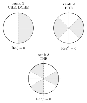
Equal-magnitude fans after a phase rotation for which $\Delta Q\sim\zeta^r$. Shading marks $\operatorname{Re}\Delta Q>0$; the dashed rays exchange exponential dominance. For CHE and the DCHE origin the actual rotation contains $\epsilon$ or $\delta$; the DCHE infinity fan has fixed phase. Lower-degree terms in BHE and THE do not change the limiting ray count.

Let

$$\mathcal B_k = \left( Y_{k,\mathrm{alg}}, Y_{k,\mathrm{exp}} \right)$$

denote analytic realizations with the prescribed formal normalizations on sector $S_k$. On an overlap, two neighboring bases are related by

$$\mathcal B_{k+1} = \mathcal B_k S_k,$$

where $S_k$ is a Stokes matrix in the chosen ordering convention. Thus the same formal symbols $\widehat Y_{\mathrm{alg}}$ and $\widehat Y_{\mathrm{exp}}$ do not define one global pair of analytic functions. The sector index may be omitted only when the domain and continuation prescription have already been fixed.

There is a second subtlety even within one sector. Where one column is exponentially dominant, adding a constant multiple of the exponentially smaller recessive column need not change the dominant column’s Poincaré series. Canonical sectorial normalization uses the summation prescription and a sufficiently wide sector, not only the leading symbol $1+O(z^{-1})$.

This book states the phase condition rather than relying on the conflicting terms “Stokes ray” and “anti-Stokes ray.” Equal magnitude does not by itself imply a nonzero Stokes multiplier.

From endpoint data to a connection problem

A dependable boundary-value statement can now be written in five lines:

1. declare the exact ODE and endpoint coordinates;
2. classify each endpoint as ordinary, regular singular, or irregular;
3. choose ordered local or sectorial bases with leading coefficient $1$;
4. record logarithm branches, angular lifts, and lateral choices;
5. verify the Wronskian against Abel’s identity.

Only then relate the two fundamental frames using the house convention,

$$\mathcal B_{\mathrm R} = \mathcal B_{\mathrm L}C_{\mathrm{LR}}.$$

The next chapter computes the entries of such connection matrices by Wronskian ratios and recurrences. This page fixes the objects being connected.

Degenerate parameters require a fresh audit

The CHE formulas at infinity assume $\epsilon\ne0$, and the DCHE formulas at $0$ assume $\delta\ne0$. If $\epsilon=0$ but $\alpha\ne0$, the CHE instead has the ramified leading factors $\exp(\pm2\sqrt{-\alpha z})$; only $\epsilon=\alpha=0$ makes infinity regular singular. If $\delta=0$, the DCHE origin has indicial polynomial $\rho(\rho-1)+\gamma\rho-q$ rather than the displayed irregular pair. The BHE origin is ordinary when $\gamma=q=0$. In every case, return to the Riccati or indicial balance and reclassify the endpoint.

Common pitfalls

A software name is not a basis declaration. Symbols such as HeunC and HeunB use package-specific parameter orders and normalizations. State the ODE and initial or asymptotic normalization before comparing values; the site’s current convention map gives worked examples.

A formal asymptotic series is not a global function. It can have distinct sectorial realizations separated by Stokes jumps. Attach a sector and a lateral prescription whenever the path meets a singular summation direction.

Resonance is not handled by blind substitution. When exponent differences become integral, a nonresonant pair may collapse and a logarithm may appear. Recompute the Levelt basis or take a controlled parameter limit.

Dominant and recessive are directional words. The inequality between two exponential magnitudes reverses across an equal-magnitude ray. Never call a solution “the decaying one” without an angular domain.

Exercises

1. Expose the ramified CHE degeneration

Set $\epsilon=0$ and $\alpha\ne0$ in the CHE. With $y=\exp(\kappa\sqrt z)z^\mu(1+o(1))$, determine $\kappa$ and $\mu$ at infinity. What happens when $\alpha=0$ as well?

Solution

The leading logarithmic derivatives are

$$\begin{aligned} \frac{y'}y &= \frac{\kappa}{2\sqrt z} +\frac{\mu}{z} +O(z^{-3/2}),\\ \frac{y''}y &= \frac{\kappa^2}{4z} +\kappa \left( \mu-\frac14 \right)z^{-3/2} +O(z^{-2}). \end{aligned}$$

When $\epsilon=0$, the CHE has $p=O(z^{-1})$ and $r=\alpha/z+O(z^{-2})$. The order-$z^{-1}$ balance is

$$\frac{\kappa^2}{4}+\alpha=0.$$

At order $z^{-3/2}$, the Riccati equation gives

$$\kappa \left( \mu-\frac14+\frac{\gamma+\delta}{2} \right) =0.$$

For either nonzero value of $\kappa$,

$$\mu = \frac14-\frac{\gamma+\delta}{2}.$$

Thus the two ramified prefactors are

$$\exp\left(\pm2\sqrt{-\alpha z}\right) z^{\,1/4-(\gamma+\delta)/2}.$$

They have centered slope $1/2$, so direct substitution into the generic $\epsilon\ne0$ atlas is invalid. If $\epsilon=\alpha=0$, then $p=O(z^{-1})$ and $r=O(z^{-2})$; infinity is regular singular.

2. Build the regular CHE germ at one

Put $x=z-1$ in the CHE and verify the first coefficient of the analytic solution normalized by $C_1(0)=1$.

Solution

Near $x=0$,

$$p=\frac{\delta}{x}+O(1), \qquad r=\frac{\alpha-q}{x}+O(1).$$

For $C_1=1+d_1x+O(x^2)$, the coefficient of $x^{-1}$ is

$$\delta d_1+\alpha-q=0.$$

Therefore

$$C_1(x) = 1+\frac{q-\alpha}{\delta}x+O(x^2).$$

3. Transport the CHE pair through a physical gauge

Let

$$R(z) = z^s(z-1)^t\exp(\kappa z)y(z).$$

Translate the generic CHE asymptotic pair into the physical variable $R$. Explain why a decay label cannot be assigned before this gauge and an angular direction are fixed.

Solution

Since $(z-1)^t\sim z^t$ on a compatible branch, the two physical prefactors are

$$\begin{aligned} R_{\mathrm{alg}} &\sim \exp(\kappa z) z^{s+t-\alpha/\epsilon},\\ R_{\mathrm{exp}} &\sim \exp\bigl((\kappa-\epsilon)z\bigr) z^{s+t+\alpha/\epsilon-\gamma-\delta}. \end{aligned}$$

The scalar gauge shifts both displayed exponentials, and their absolute decay depends on $\operatorname{Re}(\kappa z)$ and $\operatorname{Re}((\kappa-\epsilon)z)$. Their relative exponential difference remains $-\epsilon z$. Therefore labels such as ingoing, outgoing, or decaying require the physical gauge, time convention, and angular domain.

4. Audit the DCHE basis at zero

For $\delta\ne0$, use $\lambda=A/z^2+B/z+\cdots$ to recover the two leading exponential parts and the power $2-\gamma$. Check the Wronskian constant.

Solution

At order $z^{-4}$,

$$A(A+\delta)=0.$$

The branch $A=0$ has no singular exponential or power. For $A=-\delta$, the $z^{-3}$ balance gives

$$\delta(2-B-\gamma)=0,$$

so $B=2-\gamma$. Since

$$\int \left( -\frac{\delta}{z^2}+\frac{2-\gamma}{z} \right)\dd z = \frac{\delta}{z}+(2-\gamma)\operatorname{Log}z,$$

the second prefactor is $\exp(\delta/z)z^{2-\gamma}$. Differentiating it shows

$$\Wr[\widehat D_{0,\mathrm{alg}}, \widehat D_{0,\mathrm{exp}}] \sim -\delta\exp(\delta/z)z^{-\gamma},$$

in agreement with Abel’s factor.

5. Count the equal-magnitude rays

Find the limiting ray angles for the CHE, BHE, and THE. Include the parameter-dependent rotation for the CHE.

Solution

Write $z=Re^{\ii\theta}$. For the CHE,

$$\operatorname{Re}(\epsilon z)=0$$

gives

$$\theta = \frac{\pi}{2}-\arg\epsilon+k\pi.$$

For the BHE,

$$\operatorname{Re}(z^2)=0 \quad\Longrightarrow\quad \theta=\frac{\pi}{4}+\frac{k\pi}{2}.$$

For the THE,

$$\operatorname{Re}(z^3)=0 \quad\Longrightarrow\quad \theta=\frac{\pi}{6}+\frac{k\pi}{3}.$$

There are respectively two, four, and six rays modulo $2\pi$.

6. Check the ordinary THE basis

Derive the first nonconstant term of $T_0$ and compute $\Wr[T_0,T_1]$ from the initial data.

Solution

At $z=0$ the THE gives

$$y''(0)-q\,y(0)=0.$$

For $T_0(0)=1$ and $T_0'(0)=0$, this yields

$$T_0(z)=1+\frac q2z^2+O(z^3).$$

The initial basis has $\Wr[T_0,T_1](0)=1$. Since $p(z)=z^2+\gamma z$, Abel’s identity gives

$$\Wr[T_0,T_1] = \exp\left( -\int_0^z(s^2+\gamma s)\,\dd s \right) = \exp\left( -\frac{z^3}{3}-\frac{\gamma z^2}{2} \right).$$

7. Diagnose a resonant basis claim

A calculation sets $\gamma=1$ in the two general-Heun formulas at $0$ and calls the result a basis. Explain the failure and state what extra normalization is needed.

Solution

At $\gamma=1$ the exponents are both $0$. The factor $z^{1-\gamma}$ becomes $1$, and the shifted parameters in the second formula return to the first normalized germ. The displayed pair is therefore not independent.

Generically the second solution contains a multiple of $f_0\operatorname{Log}z$. One must choose a branch of $\operatorname{Log}z$ and fix the logarithmic coefficient together with the remaining freedom to add $f_0$, or specify a parameter derivative or limiting prescription that does so.

References

• NIST DLMF §31.3, especially 31.3.1 and 31.3.5, defines the normalized general-Heun local solutions and discusses their resonant restrictions.
• NIST DLMF §31.12 fixes the four confluent equations and their singularity ranks; §31.13 gives curated references for their asymptotics near irregular singularities.
• NIST DLMF §2.7(i) gives the underlying Frobenius theory, while §2.7(ii) treats rank-one irregular asymptotics. Wasow below supplies the general higher-rank sectorial existence theory used for BHE and THE.
• A. Ronveaux, ed., Heun’s Differential Equations, Oxford University Press (1995), book record and DOI, Part A, pp. 36–41 for local solutions; CHE asymptotics, pp. 120–127, DCHE analytic theory, pp. 144–166, BHE solutions, pp. 203–213, and THE singularity solutions, pp. 266–276. Parts B–E use canonical forms that require a crosswalk before their parameters are compared directly with the DLMF reduced equations.
• S. Yu. Slavyanov and W. Lay, Special Functions: A Unified Theory Based on Singularities, Oxford University Press (2000), Chapter 3, pp. 97–162.
• W. Wasow, Asymptotic Expansions for Ordinary Differential Equations, Interscience (1965), contents and edition record, especially pp. 49–87 on irregular singular points, asymptotic solutions, and the Stokes phenomenon.