Irregular Blocks and Confluent-Heun Connection Problems

Confluence changes the kind of connection problem. At a regular endpoint, a Frobenius series and its leading coefficient select a local solution. At a rank-one irregular endpoint, a formal exponential series selects an analytic solution only after one also chooses a sector, branches, and a summation prescription. The conformal-block language reflects this change: a first-kind block is adapted to a regular end, whereas a second-kind block is adapted to an irregular end.

The regular-to-irregular confluent-Heun coefficient is consequently not one universal matrix. It is a family of sector-labelled matrices. Its local irregular kernel is the same gamma-function kernel that connects Whittaker $M$ and $W$ solutions, but a nonrigid confluent-Heun problem also contains an intermediate-channel sum and derivatives of a classical irregular block.

The four-way distinction

Object	What it fixes
Rank-one irregular state	Virasoro moments of the collided insertion
First-kind irregular block	Expansion adapted to a regular endpoint
Second-kind irregular block	Sectorial expansion adapted to the irregular endpoint
Stokes matrix	Change between adjacent sectorial infinity frames

The Whittaker kernel $\mathcal N$ below is a regular-to-irregular connection kernel. It is not a Stokes multiplier.

Status of the construction

Ingredient	Status
Confluent-Heun gauge and parameter dictionary	Exact algebra
Local Frobenius recurrences and formal infinity recurrence	Exact
Finite degenerate fusion kernel $\mathcal M$	Exact
Whittaker kernel $\mathcal N$	Exact after fixing branches and a sector
Finite-$c$ second-kind blocks and their Stokes transformations	Constructed under Lenells–Roussillon Assumptions 5.1–5.2; their BPZ reduction also uses Assumption 7.1
Classical irregular-block exponentiation	Semiclassical ansatz, coefficientwise/formal in the use made here
Small-$L$ block-basis factorization	Formal consequence of fusion, collision, and the derivative-compatible semiclassical ansatz, after the Wronskian sign convention audited below
Regular-to-regular confluent-Heun formula	Independently obtained as a perturbative ODE connection expansion
Generic regular-to-irregular confluent-Heun formula	Sector-dependent CFT construction; no comparably general ODE-side proof is presently used here
Equality of the small-$L$ and large-$L$ charts	Not asserted

The exact kernels should therefore not be confused with an unconditional global theorem about the classical-block dressing around every value of $L$.

Fix the confluent-Heun gauge before naming blocks

Use the standard confluent-Heun equation

$$\begin{aligned} 0={}& y''(z) + \left( \frac{\gamma}{z} + \frac{\delta}{z-1} + \epsilon \right)y'(z) \\ &+ \frac{\alpha z-q}{z(z-1)}y(z), \qquad \epsilon\neq0. \end{aligned}$$

Set

$$\begin{aligned} y(z)&=P(z)\psi(z), \\ P(z) &= e^{-\epsilon z/2} z^{-\gamma/2} (1-z)^{-\delta/2}. \end{aligned}$$

Thus $y=P\psi$, not $\psi=P y$. The centered parameters are

$$\begin{aligned} a_0&=\frac{1-\gamma}{2}, & a_1&=\frac{1-\delta}{2}, \\ m&= \frac{\alpha}{\epsilon} - \frac{\gamma+\delta}{2}, & L&=\epsilon, \end{aligned}$$

and the normal-form accessory coordinate is

$$\begin{aligned} u ={}& \frac14-q+\alpha - \frac{ \left( \gamma+\delta-1 \right)^2 }{4} - \frac{\delta\epsilon}{2}. \end{aligned}$$

Equivalently,

$$\begin{aligned} \alpha &= L \left( m+\frac{\gamma+\delta}{2} \right), \\ q &= \frac14 - \frac{ \left( \gamma+\delta-1 \right)^2 }{4} \\ &\quad + L \left( m+\frac{\gamma}{2} \right) -u. \end{aligned}$$

The normal-form equation is

$$\begin{aligned} 0={}& \psi''(z) + \left[ \frac{\frac14-a_0^2}{z^2} + \frac{\frac14-a_1^2}{(z-1)^2} \right. \\ &\left. + \frac{ u-\frac12+a_0^2+a_1^2 }{ z(z-1) } + \frac{mL}{z} - \frac{L^2}{4} \right]\psi(z). \end{aligned}$$

This repeats only the dictionary needed on this page. The irregular-state page derives it from the BPZ equation and from the general-Heun collision.

Assume initially that

$$1-\gamma\notin\mathbb Z, \qquad 1-\delta\notin\mathbb Z,$$

and stay away from the gamma-function and internal Gram-matrix polar divisors. Resonant limits require logarithmic bases and are postponed to page 7.

Regular ends and the irregular end need different frames

At $z=0$, order the unit-leading standard-form germs as

$$\boldsymbol H_0 = \left( H_{0,-},H_{0,+} \right),$$

where

$$\begin{aligned} H_{0,-}(z) &= 1+O(z), \\ H_{0,+}(z) &= z^{1-\gamma} \left[ 1+O(z) \right]. \end{aligned}$$

At $z=1$, put $x=1-z$ and use

$$\boldsymbol H_1 = \left( H_{1,-},H_{1,+} \right),$$

with

$$\begin{aligned} H_{1,-}(z) &= 1+O(x), \\ H_{1,+}(z) &= x^{1-\delta} \left[ 1+O(x) \right]. \end{aligned}$$

Both frames are ordinary Frobenius frames. Their precise $\operatorname{HeunC}$ parameter transformations follow from $z\mapsto1-z$; the Heun confluence page records the singularity pattern and coefficient limit.

Infinity is different. Its two formal standard-form branches are

$$\begin{aligned} \widehat Y_+(z) &= z^{-\alpha/\epsilon} \left[ 1+\frac{c_1}{z}+O(z^{-2}) \right], \\ \widehat Y_-(z) &= e^{-\epsilon z} z^{\alpha/\epsilon-\gamma-\delta} \left[ 1+O(z^{-1}) \right], \end{aligned}$$

where

$$\begin{aligned} c_1 = \frac{ \alpha^2 - (\gamma+\delta-1)\alpha\epsilon + (\alpha-q)\epsilon^2 }{ \epsilon^3 }. \end{aligned}$$

The exponent difference contains $-\epsilon z$. Equal magnitude occurs on

$$\operatorname{Re}(\epsilon z)=0.$$

Consequently, an unsuffixed symbol such as $\operatorname{HeunC}_{\infty}$ is incomplete. Choose:

1. a branch of $\Log z$ and $\Log L$;
2. a continuation path from the regular endpoint;
3. a sector $\Sigma_k$ whose interior avoids the relevant singular summation directions;
4. a lateral or summation prescription.

The equal-magnitude rays $\operatorname{Re}(\epsilon z)=0$ locate dominance changes, whereas Stokes jumps are tied to singular summation directions. Because the two ray-naming conventions are reversed in parts of the literature, this book states the phase condition rather than using “Stokes ray” for both.

Only then denote the analytic realizations by

$$\boldsymbol Y_\infty^{(k)} = \left( Y_+^{(k)},Y_-^{(k)} \right).$$

In normal form, their leading behaviors are

$$\begin{aligned} \psi_{\infty,+}^{(k)}(z) &\sim e^{Lz/2}z^{-m}, \\ \psi_{\infty,-}^{(k)}(z) &\sim e^{-Lz/2}z^{m}. \end{aligned}$$

Multiplication by $P$ recovers the algebraic and exponentially small or large standard-form branches above.

First-kind blocks live at regular endpoints

Let

$$F=F(a,a_0,a_1,m;L)$$

be the reduced small-$L$ classical irregular block, with the leading internal power separated:

$$f_{\mathrm{irr}} = \left( \frac14-a^2 \right)\Log L +F.$$

The accessory relation is

$$u = \frac14-a^2 + L\partial_LF.$$

This relation is inverted locally to obtain $a=a(q)$ on a chosen lift. The inverse requires

$$\partial_a u\neq0.$$

All derivatives below are partial derivatives of the reduced $F$ at fixed $L$, fixed remaining momenta, and fixed branches. Write

$$F_0=\partial_{a_0}F, \qquad F_1=\partial_{a_1}F, \qquad F_a=\partial_aF, \qquad F_m=\partial_mF.$$

After division by the background block, the degenerate first-kind blocks at the regular ends have leading behaviors

$$\begin{aligned} B_{0,s}(z) &= e^{-sF_0/2} z^{1/2+s a_0} \left[ 1+O(z,L) \right], \\ B_{1,s}(z) &= e^{-sF_1/2} (1-z)^{1/2+s a_1} \left[ 1+O(1-z,L) \right], \end{aligned}$$

where the sign labels $s=-,+$ are read as the numerical values $s=-1,+1$ inside formulas. These are normal-form solutions. “First kind” describes the expansion at a regular singular point even though the background state at infinity is irregular.

For the initial regular-to-regular relation, take $0<z<1$, make $\Log z$ and $\Log(1-z)$ real, and continue without winding around either endpoint. The block relation uses the same local degenerate fusion kernel as the hypergeometric problem:

$$B_{0,s} = \sum_{r=\pm} \mathcal M_{sr}(a_0,a_1;a) B_{1,r},$$

where

$$\begin{aligned} \mathcal M_{sr}(x,y;h) = \frac{ \Gamma(-2r y) \Gamma(1+2s x) }{ \Gamma\left( \frac12+s x-r y+h \right) \Gamma\left( \frac12+s x-r y-h \right) }. \end{aligned}$$

The kernel is exact. Turning this block relation into a unit-leading standard-form matrix still requires the scalar gauge and endpoint normalizations.

A normalization check at one

Near $z=1$ on the chosen branch,

$$P(z) \sim e^{-L/2} (1-z)^{-\delta/2}.$$

Therefore the unit-leading standard-form germs are related to the block representatives by

$$\begin{aligned} H_{1,s} = e^{L/2} P(z) e^{sF_1/2} B_{1,s}. \end{aligned}$$

The common $e^{L/2}$ is forced by the value of the exponential gauge at the endpoint. Dropping it changes every regular-to-one coefficient and violates the Abel–Wronskian determinant. This small audit is one reason to keep block relations and unit-leading ODE matrices distinct.

Apparent normalization inconsistencies in the printed formula

The standard-form translation in Bonelli et al., Eq. (4.2.18), appears to omit this common endpoint factor. Its two printed infinity functions also use the argument $z$, whereas their defining inverse-power series requires $z^{-1}$. These are treated here as apparent transcription or normalization inconsistencies, not as an official erratum. The next page derives the unit-leading matrix from the local frames instead of copying that displayed formula.

Second-kind blocks are sectorial

Move the degenerate probe toward the irregular state instead. The result is a second-kind block. In the small-$L$ chart, its classical normal-form representative in sector $\Sigma_k$ behaves as

$$\begin{aligned} D_r^{(k)}(z) ={}& e^{-rF_m/2} e^{rLz/2} L^{-1/2-rm} z^{-rm} \\ &\times \left[ 1+ O\left( L,\frac1{Lz} \right) \right], \qquad r=\pm. \end{aligned}$$

This is not a convergent Frobenius germ on a punctured disk. It is an asymptotic object attached to a sector. The power $L^{-1/2-rm}$, the branch of $z^{-rm}$, and the lateral realization of the formal series are all part of its normalization.

For an upper or lower continuation to a large positive-$z$ ray, encode the lateral choice by $\eta=\pm1$ and take

$$\arg(1-z)=-\eta\pi.$$

Then the unit-leading standard-form infinity functions satisfy

$$\begin{aligned} Y_r^{(\eta)} ={}& e^{-\eta\ii\pi\delta/2} P(z) e^{rF_m/2} L^{1/2+rm} D_r^{(\eta)}. \end{aligned}$$

The phase comes from

$$(1-z)^{-\delta/2} \sim e^{\eta\ii\pi\delta/2} z^{-\delta/2}.$$

Changing the lateral path changes this phase and may also cross a Stokes ray. A phase choice is not a substitute for the sector label.

The Whittaker kernel is exact

Before treating the nonrigid confluent-Heun equation, isolate the rigid local kernel. Whittaker’s equation is

$$\frac{\dd^2w}{\dd x^2} + \left[ -\frac14 + \frac{m}{x} + \frac{\frac14-a^2}{x^2} \right]w =0.$$

For $2a\notin\mathbb Z$, its regular branches are $M_{m,s a}(x)$ with $s=\pm$. Fix an unwrapped argument in

$$-\frac{\pi}{2} < \arg x < \frac{3\pi}{2},$$

and use

$$\Log\left(e^{-\ii\pi}x\right) = \Log x-\ii\pi.$$

One sectorial infinity pair is

$$\begin{aligned} W_+(x) &= e^{-\ii\pi m} W_{-m,a} \left( e^{-\ii\pi}x \right), \\ W_-(x) &= W_{m,a}(x). \end{aligned}$$

Substitute $\mu=s a$ into the standard $M$–$W$ connection identity and use $W_{m,a}=W_{m,-a}$. On the declared continuation branch this gives

$$M_{m,s a}(x) = \sum_{r=\pm} \mathcal N_{sr}(a,m) W_r(x),$$

with

$$\begin{aligned} \mathcal N_{sr}(a,m) ={}& \frac{ \Gamma(1+2s a) }{ \Gamma\left( \frac12+s a-rm \right) } \\ &\times \exp\left[ \ii\pi \frac{1-r}{2} \left( \frac12-m+s a \right) \right]. \end{aligned}$$

Thus

$$\begin{aligned} \mathcal N_{s,+} &= \frac{ \Gamma(1+2s a) }{ \Gamma\left( \frac12+s a-m \right) }, \\ \mathcal N_{s,-} &= \frac{ \Gamma(1+2s a) }{ \Gamma\left( \frac12+s a+m \right) } e^{\ii\pi(1/2-m+s a)}. \end{aligned}$$

This identity is an exact special-function connection formula, extended meromorphically away from the initially generic domain. It supplies the local irregular core of the confluent-Heun problem. Its phase records the clockwise determination $e^{-\ii\pi}x$.

The small-L map factors through an overlap region

For

$$|L|\ll1,$$

there is an overlap region in which the regular punctures are far away but the irregular exponential has not yet become large:

$$1\ll |z|\ll |L|^{-1}.$$

The continuation from $z=1$ to infinity can be organized in two local operations:

1. use a regular fusion kernel $\mathcal M$ to reach the intermediate channel $\sigma=\pm$;
2. use the Whittaker kernel $\mathcal N$ to enter the chosen irregular sector.

The direct collision formula first produces the raw kernel

$$\begin{aligned} \left( K_{\mathrm{raw}}^{(k)} \right)_{sr} ={}& \sum_{\sigma=\pm} \mathcal M_{s\sigma}(a_1,a;a_0) \mathcal N_{-\sigma,r}^{(k)}(a,m) \\ &\qquad\times L^{\sigma a} \exp\left( -\frac{\sigma}{2}F_a \right). \end{aligned}$$

The sector label on $\mathcal N$ reminds us that its phase convention is not universal. In the branch fixed in the preceding section,

$$\begin{aligned} \left( K_{\mathrm{raw}} \right)_{sr} ={}& \sum_{\sigma=\pm} \frac{ \Gamma(1+2s a_1) \Gamma(-2\sigma a) \Gamma(1-2\sigma a) }{ \Gamma\left( \frac12+s a_1-\sigma a+a_0 \right) } \\ &\times \frac{ e^{\ii\pi(1-r)(1/2-m-\sigma a)/2} L^{\sigma a} e^{-\sigma F_a/2} }{ \Gamma\left( \frac12+s a_1-\sigma a-a_0 \right) \Gamma\left( \frac12-\sigma a-rm \right) }. \end{aligned}$$

A one-column sign is fixed by the Wronskian

The raw formula has an apparent sign inconsistency if it is attached directly to the unit-leading frames declared above. Gamma reflection identities give

$$\det\mathcal M(a_1,a;a_0) = -\frac{a_1}{a},$$

and, with row order $\sigma=(-,+)$ and column order $r=(+,-)$,

$$\det \left[ \mathcal N_{-\sigma,r} \right] = 2a.$$

The diagonal factors $L^{\sigma a}e^{-\sigma F_a/2}$ have determinant one. Hence

$$\det K_{\mathrm{raw}} = -2a_1.$$

On the other hand, the declared leading terms give

$$\begin{aligned} \operatorname{Wr} \left[ B_{1,-},B_{1,+} \right] &= -2a_1 \left[ 1+O(L) \right], \\ \operatorname{Wr} \left[ D_+,D_- \right] &= -1 \left[ 1+O(L) \right]. \end{aligned}$$

The exact Wronskians are constant in $z$; the displayed $O(L)$ terms record the remaining diagonal small-$L$ block normalizations, which are assembled on page 6. In particular, a relation $\boldsymbol B_1=\boldsymbol D_\infty K^{\mathsf T}$ requires a positive leading determinant $2a_1$, not the negative value of $K_{\mathrm{raw}}$.

Introduce the collision-frame sign

$$J_\infty = \operatorname{diag}(1,-1), \qquad \det J_\infty=-1,$$

and define the Wronskian-normalized coefficient by

$$K^{(k)} = K_{\mathrm{raw}}^{(k)}J_\infty.$$

Its leading determinant is $2a_1$. The diagonal analytic normalizations suppressed by the $O(L)$ notation are separate from this relative sign.

Equivalently, multiply the $r=-$ column of the expanded gamma sum by $-1$. Choosing instead $J_\infty=\operatorname{diag}(-1,1)$ differs by a common sign of the regular block frame. The relative sign is fixed; that harmless common frame sign is not.

This $J_\infty$ exposes an apparent one-column sign ambiguity in the printed collision formula. It does not modify the exact Whittaker identity for the explicitly defined pair $(W_+,W_-)$; it fixes the identification of that pair with the published second-kind block frame.

The Wronskian-normalized block-basis connection relation is

$$B_{1,s} = \sum_{r=\pm} K_{sr}^{(k)} D_r^{(k)}.$$

With the row-frame orders

$$\boldsymbol B_1 = \left( B_{1,-},B_{1,+} \right), \qquad \boldsymbol D_\infty^{(k)} = \left( D_+^{(k)},D_-^{(k)} \right),$$

the same relation reads

$$\boldsymbol B_1 = \boldsymbol D_\infty^{(k)} \left( K^{(k)} \right)^{\mathsf T}.$$

The transpose is not decoration: $s$ labels the regular source and $r$ the irregular target. The intermediate sign $\sigma$ labels two ways of reaching the same two-dimensional solution space; it is not a third local solution. The determinant audit also makes the hidden collision-frame sign independently checkable.

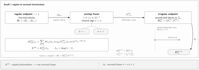
For small $L$, a regular-to-irregular map factors through the overlap channel: $\mathcal M$ performs regular degenerate fusion and $\mathcal N^{(k)}$ performs the Whittaker-type entry into sector $\Sigma_k$. The sign $J_\infty$ aligns the printed collision kernel with the declared unit-leading Wronskians. The separate arrow $S_k$ changes sectorial infinity frames; it is not part of the definition of $\mathcal N^{(k)}$.

What the factorization does and does not prove

The finite-$c$ fusion and Whittaker kernels are exact. The displayed classical dressing follows after assuming:

• exponentiation of the selected irregular background block;
• derivative-compatible heavy–light factorization;
• compatibility of the collision limit with analytic continuation;
• a fixed branch of the accessory-to-Floquet inverse $a(q)$;
• a fixed sectorial realization at infinity.

Under these hypotheses it is an all-orders identity of the relevant formal small-$L$ expansions. It should not be advertised as one single-valued expression valid after unrestricted continuation in $L$.

Stokes matrices change the sector, not the endpoint

Let adjacent row frames satisfy the book convention

$$\boldsymbol D_\infty^{(k+1)} = \boldsymbol D_\infty^{(k)}S_k.$$

The Stokes matrix $S_k$ is triangular and unipotent after a compatible ordering by dominance. It relates two analytic realizations of the same formal infinity basis.

If

$$\boldsymbol B_1 = \boldsymbol D_\infty^{(k)} C_{\infty1}^{(k)},$$

then the same regular frame expressed in the adjacent sector obeys

$$C_{\infty1}^{(k+1)} = S_k^{-1} C_{\infty1}^{(k)}.$$

This transformation law sharply separates the two roles:

$$\begin{array}{c|c} \mathcal N^{(k)} & \text{regular or intermediate frame} \longrightarrow \text{one sectorial infinity frame} \\ S_k & \text{sectorial infinity frame }k \longrightarrow \text{sectorial infinity frame }k+1 \end{array}$$

Formal monodromy is a third operation. Under $\Log z\mapsto\Log z+2\pi\ii$, the standard-form formal powers give

$$M_{\mathrm f} = \operatorname{diag} \left( e^{-2\pi\ii\alpha/\epsilon}, e^{2\pi\ii(\alpha/\epsilon-\gamma-\delta)} \right).$$

The actual monodromy at the irregular point is assembled from formal monodromy and the ordered product of Stokes matrices. Neither one alone is the regular-to-irregular connection matrix.

Small-L and large-L blocks are different charts

There are two independent distinctions:

Question	Alternatives
Where is the degenerate probe expanded?	Regular end: first kind; irregular end: second kind
Which scale chart describes the background?	Small $L$: expansion in $L$; large $L$: expansion in $L^{-1}$

Thus “second kind” is not merely another name for “large $L$.” A small-$L$ background can still carry a second-kind degenerate probe near infinity, as in the factorization above.

In the large-$L$ chart, introduce a different internal parameter $m'$ and a dual classical block

$$F_D=F_D(a_0,a_1,m,m';L^{-1}).$$

Its accessory relation begins

$$\begin{aligned} u_D ={}& -(m'-m)L + \frac14-a_0^2 \\ &+ 2m'(m'-m) + O(L^{-1}). \end{aligned}$$

$u_D$ is the same accessory coordinate $u$ represented in the large-$L$ chart, not a second accessory parameter. One now inverts this relation for $m'=m'(q)$ rather than for $a=a(q)$, on a branch where

$$\partial_{m'}u_D\ne0.$$

The natural large-$L$ block representatives are fixed by the local normalizations

$$\begin{aligned} \mathcal D_{1,s}(z) \sim{}& L^{s a_1} \exp\left( -\frac{s}{2}\partial_{a_1}F_D \right) (1-z)^{1/2+s a_1} \\ &\times \left[ 1+O\left( L^{-1},L(1-z) \right) \right], \end{aligned}$$

and

$$\begin{aligned} \mathcal D_{\infty,r}^{(k)}(z) \sim{}& e^{rLz/2}e^{-rL/2} \exp\left( -\frac{r}{2}\partial_mF_D \right) \\ &\times L^{-1/2+r(m'-m)} z^{-rm} \left[ 1+O\left( L^{-1},z^{-1} \right) \right]. \end{aligned}$$

Here $s,r=\pm1$, all powers use the declared logarithms, and the infinity asymptotic is read inside the chosen sector $\Sigma_k$. These leading forms make clear which powers and block derivatives must later be removed to obtain unit-leading standard functions.

The large-$L$ block-basis connection from a regular end to infinity has the simpler local anatomy

$$\mathcal D_{1,s} = \sum_{r=\pm} \mathcal N_{s,-r} \left( a_1,m'-m \right) \mathcal D_{\infty,r}^{(k)}.$$

The simplicity is chart-dependent. Converting this relation to unit-leading standard-form functions still supplies powers of $L$, endpoint gauges, derivatives of $F_D$, and lateral phases.

The two expansions may describe analytic continuations of the same differential equation after suitable resummation, but their formal series, internal coordinates, and natural normalizations are different. One must not insert a small-$L$ $a(q)$ into a large-$L$ formula or infer $F_D$ by replacing $L$ with $L^{-1}$ in $F$.

An exact removable-puncture benchmark

The local irregular kernel, its lateral phase, and the matrix direction can all be tested without a semiclassical assumption. Take

$$\left( \gamma,\delta,\epsilon,\alpha,q \right) = \left( \frac43,0,-1,-\frac5{12},-\frac5{12} \right).$$

Both conditions

$$\delta=0, \qquad q=\alpha$$

are needed to remove $z=1$. The equation becomes

$$z y'' + \left( \frac43-z \right)y' - \frac5{12}y =0,$$

which is Kummer’s equation with

$$a_{\mathrm K}=\frac5{12}, \qquad b_{\mathrm K}=\frac43.$$

Equivalently, its Whittaker parameters are

$$\kappa=\frac14, \qquad \mu=\frac16.$$

The centered confluent-Heun dictionary gives $L=-1$ and $m=-1/4$. With the Whittaker coordinate $x=-Lz=z$, its parameters are therefore

$$\left( a_{\mathrm W},m_{\mathrm W},x \right) = \left( \frac16,\frac14,-Lz \right),$$

so that $a_{\mathrm W}=\mu$ and $m_{\mathrm W}=\kappa=-m$. This sign comes from the change of asymptotic coordinate, not from a change in the original confluent-Heun parameters.

On one fixed branch of $\Log z$, put

$$h(z) = e^{z/2}z^{-2/3}.$$

Use the unit-leading regular frame

$$\begin{aligned} R_+(z) &= h(z)M_{\kappa,\mu}(z) = {}_1F_1 \left( \frac5{12};\frac43;z \right), \\ R_-(z) &= h(z)M_{\kappa,-\mu}(z) \\ &= z^{-1/3} {}_1F_1 \left( \frac1{12};\frac23;z \right). \end{aligned}$$

The down arrow below labels the clockwise, or lower, determination of the rotated argument $-z$; it does not say that $z$ lies in the lower half-plane. Take

$$0<\arg z<\pi, \qquad \Log(e^{-\ii\pi}z) = \Log z-\ii\pi,$$

and define the sectorial infinity frame

$$\begin{aligned} D_0(z) &= h(z)W_{\kappa,\mu}(z) \sim z^{-5/12}, \\ D_1^\downarrow(z) &= e^{-\ii\pi\kappa} h(z) W_{-\kappa,\mu} \left( e^{-\ii\pi}z \right) \\ &\sim e^z z^{-11/12}. \end{aligned}$$

For the row frames

$$\boldsymbol R = \left( R_+,R_- \right), \qquad \boldsymbol D^\downarrow = \left( D_0,D_1^\downarrow \right),$$

the notation matches the general frame orders by

$$\left( R_+,R_- \right) = \left( H_{0,-},H_{0,+} \right), \qquad \left( D_0,D_1^\downarrow \right) = \left( Y_+,Y_- \right).$$

The exact connection relation is

$$\boldsymbol R = \boldsymbol D^\downarrow C^\downarrow,$$

with

$$\begin{aligned} C^\downarrow = \begin{pmatrix} \displaystyle \frac{ \Gamma(4/3)e^{5\pi\ii/12} }{ \Gamma(11/12) } & \displaystyle \frac{ \Gamma(2/3)e^{\pi\ii/12} }{ \Gamma(7/12) } \\ \displaystyle \frac{ \Gamma(4/3) }{ \Gamma(5/12) } & \displaystyle \frac{ \Gamma(2/3) }{ \Gamma(1/12) } \end{pmatrix}. \end{aligned}$$

The upper continuation replaces the two displayed exponential phases by their conjugates. Its exponential solution $D_1^\uparrow$ is related to the lower one by

$$\boldsymbol D^\uparrow = \boldsymbol D^\downarrow S, \qquad S = \begin{pmatrix} 1&s_{\mathrm W}\\ 0&1 \end{pmatrix},$$

where

$$s_{\mathrm W} = \frac{ 2\pi\ii }{ \Gamma(11/12)\Gamma(7/12) } \approx 3.8938354371\ii.$$

Accordingly,

$$C^\downarrow = S C^\uparrow.$$

This is the concrete version of the abstract sector law above. The regular frame did not change; the infinity frame did.

Two independent checks

Abel’s identity gives

$$\begin{aligned} \operatorname{Wr} \left[ R_+,R_- \right] &= -\frac13 e^z z^{-4/3}, \\ \operatorname{Wr} \left[ D_0,D_1^\downarrow \right] &= e^z z^{-4/3}. \end{aligned}$$

Therefore

$$\det C^\downarrow = -\frac13.$$

The gamma matrix gives the same value exactly.

At

$$z_* = 3e^{\ii\pi/4},$$

direct 60-digit evaluation yields

$$\begin{aligned} D_0(z_*) &\approx 0.5957434792 - 0.1981407874\ii, \\ D_1^\downarrow(z_*) &\approx 1.1208360751 + 3.0662463577\ii, \\ R_+(z_*) &\approx 0.7627936519 + 1.7304008913\ii, \\ R_-(z_*) &\approx 0.6871335707 + 0.3281155303\ii. \end{aligned}$$

The maximum value and derivative residuals in $\boldsymbol R-\boldsymbol D^\downarrow C^\downarrow$ are respectively $3.9\times10^{-61}$ and $1.6\times10^{-61}$; the determinant error is $3.9\times10^{-62}$.

The reproducibility script performs the value, derivative, determinant, and matrix Stokes checks with mpmath. Its declared benchmark domain is $|z_*|>0$ and $0<\arg z_*<\pi$. This slice audits the gamma core, gauge, matrix direction, lateral phase, and Stokes normalization. Because $z=1$ is removable, it does not test the generic accessory-block dressing.

A normalization-aware workflow

For a concrete confluent-Heun connection problem:

1. Fix $(q,\alpha,\gamma,\delta,\epsilon)$ and the gauge $y=P\psi$.
2. Compute $(a_0,a_1,m,L,u)$ from the exact dictionary.
3. Choose the small-$L$ or large-$L$ accessory chart.
4. Invert the appropriate accessory relation for $a(q)$ or $m'(q)$.
5. Declare $\Log L$, $\Log z$, the continuation path, and the infinity sector.
6. Evaluate the finite kernels $\mathcal M$ and $\mathcal N^{(k)}$.
7. Dress them with the appropriate derivatives of $F$ or $F_D$.
8. Convert block representatives to the declared unit-leading ODE frames, retaining endpoint values of the scalar gauge.
9. Check the matrix direction and determinant with Wronskians.
10. Continue to an adjacent sector only by applying the corresponding Stokes matrix.

The next page performs step 8 systematically and explains which subleading or normalization data survive when one passes from a classical block to a full connection coefficient.

Common pitfalls

Calling every irregular block “second kind.” A first-kind block may have an irregular background but is expanded at a regular endpoint. Second kind refers to an expansion at the irregular endpoint itself.

Calling $\mathcal N$ a Stokes matrix. $\mathcal N$ connects a regular or intermediate basis to one sectorial infinity basis. A Stokes matrix compares two adjacent infinity bases.

Writing an infinity function without a sector. The formal series does not select a unique analytic function. Supply a sector, a branch, and a lateral or summation prescription.

Equating small $L$ with first kind. The location kind and the scale chart are independent classifications.

Dropping the endpoint value of the gauge. At $z=1$, $e^{-Lz/2}\to e^{-L/2}$. Omitting this constant changes the connection matrix even though it does not change the differential equation.

Treating $a$ as an independent CHE parameter after fixing $q$. $a$ is a lifted Floquet coordinate obtained by locally inverting the accessory relation. Its branch and the condition $\partial_a u\neq0$ must be stated.

Using a small-L series at strong coupling. The $F$ and $F_D$ charts have different internal coordinates and asymptotic normalizations.

Reading every gamma pole as a divergent physical answer. At resonance, individual generic-basis entries can diverge while a logarithmic or meromorphically renormalized matrix has a finite limit.

Exercises

1. Recover the standard-form infinity powers

Starting from

$$\psi_{\infty,r} \sim e^{rLz/2}z^{-rm},$$

multiply by $P$ and recover the two formal powers of the standard confluent-Heun equation.

Solution

For large $z$,

$$P(z) \sim e^{-Lz/2} z^{-(\gamma+\delta)/2} \times \text{a branch phase}.$$

For $r=+$,

$$\begin{aligned} P\psi_{\infty,+} &\sim z^{-m-(\gamma+\delta)/2} \\ &= z^{-\alpha/\epsilon}. \end{aligned}$$

For $r=-$,

$$\begin{aligned} P\psi_{\infty,-} &\sim e^{-Lz} z^{m-(\gamma+\delta)/2} \\ &= e^{-\epsilon z} z^{\alpha/\epsilon-\gamma-\delta}. \end{aligned}$$

The omitted scalar phase is fixed by the branch of $1-z$.

2. Derive the endpoint factor at one

Use the leading behavior of $B_{1,s}$ and $P$ to show that $H_{1,s}$ needs the common factor $e^{L/2}$.

Solution

Since

$$\frac{\delta}{2} = \frac12-a_1,$$

one has

$$\begin{aligned} P B_{1,s} \sim{}& e^{-L/2} e^{-sF_1/2} \\ &\times (1-z)^{a_1+s a_1}. \end{aligned}$$

For $s=-$, the power is zero; for $s=+$, it is $2a_1=1-\delta$. Multiplying by $e^{L/2}e^{sF_1/2}$ produces the two unit-leading standard-form germs.

3. Expand the two-step kernel

Insert the definitions of $\mathcal M$ and $\mathcal N$ into $K_{sr}$ and recover the displayed three-denominator gamma sum.

Solution

Use

$$\begin{aligned} \mathcal M_{s\sigma}(a_1,a;a_0) ={}& \frac{ \Gamma(-2\sigma a) \Gamma(1+2s a_1) }{ \Gamma(\frac12+s a_1-\sigma a+a_0) } \\ &\times \frac1{ \Gamma(\frac12+s a_1-\sigma a-a_0) }, \end{aligned}$$

and

$$\begin{aligned} \mathcal N_{-\sigma,r}(a,m) ={}& \frac{ \Gamma(1-2\sigma a) }{ \Gamma(\frac12-\sigma a-rm) } \\ &\times e^{\ii\pi(1-r)(1/2-m-\sigma a)/2}. \end{aligned}$$

Multiplication and summation over $\sigma=\pm$ give exactly the displayed formula for $K_{sr}$.

4. Propagate a sector change

Suppose

$$\boldsymbol D_\infty^{(k+1)} = \boldsymbol D_\infty^{(k)}S_k$$

and

$$\boldsymbol B_1 = \boldsymbol D_\infty^{(k)} C_{\infty1}^{(k)}.$$

Find $C_{\infty1}^{(k+1)}$.

Solution

Substitute

$$\boldsymbol D_\infty^{(k)} = \boldsymbol D_\infty^{(k+1)}S_k^{-1}$$

into the second relation. Then

$$\boldsymbol B_1 = \boldsymbol D_\infty^{(k+1)} S_k^{-1}C_{\infty1}^{(k)},$$

so

$$C_{\infty1}^{(k+1)} = S_k^{-1}C_{\infty1}^{(k)}.$$

5. Explain the overlap region

Why does the small-$L$ factorization use $1\ll|z|\ll|L|^{-1}$?

Solution

The first inequality puts the probe far from the two regular punctures, so the intermediate channel is natural. The second gives $|Lz|\ll1$, so the irregular exponential can still be matched to its small-argument Whittaker representation. The two conditions can hold simultaneously only when $|L|\ll1$.

6. Separate the two classifications

Classify each object by endpoint kind and scale chart: $B_{0,s}$, $D_r^{(k)}$, and a regular-end block normalized by $F_D$.

Solution

• $B_{0,s}$ is first kind and belongs to the small-$L$ chart.
• $D_r^{(k)}$ is second kind at infinity but, in the formula on this page, is normalized by the small-$L$ background.
• A regular-end block normalized by $F_D$ is first kind with respect to the probe location and belongs to the large-$L$ chart.

This shows why “first/second kind” and “small/large $L$” cannot be used as synonyms.

References

• G. Bonelli, C. Iossa, D. Panea Lichtig, and A. Tanzini, “Irregular Liouville Correlators and Connection Formulae for Heun Functions”, Communications in Mathematical Physics 397 (2023), 635–727. Section 2.2 gives the exact Whittaker blocks and kernel; Section 3.2 constructs the confluent blocks and their semiclassical limits; Section 4.2 translates them to the confluent-Heun equation.
• J. Lenells and J. Roussillon, “Confluent Conformal Blocks of the Second Kind”, Journal of High Energy Physics 2020 (6), 133. Theorems 1 and 2 construct first-to-second-kind connection kernels and Stokes transformations under Assumptions 5.1–5.2; the BPZ specialization additionally uses Assumption 7.1 and recovers the Whittaker sectorial problem.
• O. Lisovyy, H. Nagoya, and J. Roussillon, “Irregular Conformal Blocks and Connection Formulae for Painlevé V Functions”, Journal of Mathematical Physics 59 (2018), 091409. Establishes the short-distance Painlevé-V expansion and develops the distinction between two types of rank-one irregular block; its asymptotic-parameter connection formula is stated conjecturally.
• O. Lisovyy and A. Naidiuk, “Perturbative Connection Formulas for Heun Equations”, Journal of Physics A: Mathematical and Theoretical 55 (2022), 434005. Theorem C gives an ODE-side perturbative construction for the confluent-Heun connection between its two Fuchsian points; the paper explicitly leaves irregular-endpoint connections for future work.
• O. Lisovyy and A. Naidiuk, “Accessory Parameters in Confluent Heun Equations and Classical Irregular Conformal Blocks”, Letters in Mathematical Physics 111 (2021), 137. Develops the large-parameter accessory chart and states its relation to second-kind classical irregular blocks as a conjecture.
• NIST Digital Library of Mathematical Functions, §31.12, “Confluent Forms of Heun’s Equation” and §13.14, “Whittaker Functions”. These fix the differential equations and standard special-function normalizations used in the exact benchmark.