Green Functions, Poles, and QNM Conditions from Recurrences

A continued fraction first answers a projective question: does the sequence selected by the left endpoint lie on the same line as the sequence selected at infinity? A Green function asks a stronger question: can an inhomogeneous source be inverted on declared spaces and boundary conditions? A quasinormal-mode claim is stronger again, because the selected sequence lines must represent the intended physical endpoint conditions on a specified analytic sheet.

This page proves the exact algebraic bridge between the first two questions. On the affine chart where the remote solution has $r_0\neq0$, the endpoint relation is the meromorphic identity

$$G_{00}(\lambda) = \frac{1}{F_0(\lambda)}.$$

The regular homogeneous form, valid through a ratio-chart failure, appears below. The formula is elementary; its interpretation is conditional. The aim is to make every condition visible in the chain

$$\begin{gathered} \text{recurrence-line intersection} \\ \Downarrow \\ \text{sequence inverse pole} \\ \Downarrow \\ \text{ODE resolvent pole} \\ \Downarrow \\ \text{QNM or response pole}. \end{gathered}$$

None of the arrows is automatic.

Three kernels and three levels of meaning

The word “Green function” is often used before its inverse problem has been specified. The following firewall will be used throughout the page.

Object	Defining problem	Natural denominator	Meaning of a pole
Sequence Green matrix	Invert an inhomogeneous recurrence with declared left and right sequence conditions	Discrete Casoratian	Failure of the sequence operator to be invertible
ODE Green kernel	Invert a differential operator or analytic pencil with a declared domain	Abel-normalized Wronskian	Pole of that operator or of its declared continuation
Source-to-response kernel	Reconstruct a measured field or response after gauge, source, and normalization maps	Boundary source coefficient or response ratio	A pole only if reconstruction and numerator factors do not cancel it

There is a further distinction inside the first row. An algebraic matrix that solves the recurrence for finitely supported sources is a formal Green matrix. It is a resolvent kernel only after one proves that it defines the inverse of a closed operator between specified spaces. On a nonphysical sheet it may instead represent a meromorphic continuation of matrix elements, not a bounded Hilbert-space resolvent.

The operator and resonance ledger supplies the domain and sheet language. Here the new work is recurrence native.

A source row splices two selected sequence lines

Let the analytic parameter be $\lambda\in\Omega$, and consider

$$\begin{aligned} \bigl(T(\lambda)u\bigr)_0 &= \alpha_0u_1+\beta_0u_0, \\ \bigl(T(\lambda)u\bigr)_n &= \alpha_nu_{n+1} +\beta_nu_n +\gamma_nu_{n-1}, \qquad n\geq1. \end{aligned}$$

The dependence on $\lambda$ is suppressed on the right. Work first on a patch on which

$$\alpha_n\gamma_{n+1}\neq0, \qquad n\geq0.$$

A structural zero that splits or terminates the recurrence must instead be handled blockwise, as on the truncation page.

Choose two homogeneous solutions:

• $\ell$ satisfies the left row and is continued to the right;
• $r$ satisfies the chosen remote condition—minimal, square summable, outgoing, or another declared analytic continuation—and is continued to the left.

Use the chapter’s Casoratian convention

$$\mathcal K_n[\ell,r] = \ell_nr_{n+1}-\ell_{n+1}r_n.$$

For a source at $m$ and away from a zero of the denominator, define

$$G_{nm} = \frac{ \ell_{\min(n,m)}r_{\max(n,m)} }{ \alpha_m\mathcal K_m[\ell,r] }.$$

The same formula then supplies the local meromorphic continuation wherever the normalized ingredients extend analytically.

Every row with $n\neq m$ is homogeneous: on the left the column is a multiple of $\ell$, and on the right it is a multiple of $r$. For $m\geq1$, the source row gives

$$\begin{aligned} \bigl(TG_{\bullet m}\bigr)_m &= \frac{ \alpha_m\ell_mr_{m+1} +\beta_m\ell_mr_m +\gamma_m\ell_{m-1}r_m }{ \alpha_m\mathcal K_m } \\ &= \frac{ \alpha_m \left( \ell_mr_{m+1}-\ell_{m+1}r_m \right) }{ \alpha_m\mathcal K_m } =1. \end{aligned}$$

The second line used the homogeneous equation for $\ell$. At $m=0$, the endpoint calculation is instead

$$\begin{aligned} \bigl(TG_{\bullet0}\bigr)_0 &= \frac{ \ell_0 \left( \alpha_0r_1+\beta_0r_0 \right) }{ \alpha_0\mathcal K_0 } \\ &= \frac{ \alpha_0 \left( \ell_0r_1-\ell_1r_0 \right) }{ \alpha_0\mathcal K_0 } =1. \end{aligned}$$

Thus

$$TG_{\bullet m}=e_m$$

as an exact algebraic identity. The jump denominator is $\alpha_m\mathcal K_m$. For $m\geq1$ it is equivalently $\gamma_m\mathcal K_{m-1}$; the endpoint has no $\gamma_0\mathcal K_{-1}$ representation. Shifting either coefficient without shifting the Casoratian is a common off-by-one error.

A weighted Casoratian removes source-index dependence

For a nonsymmetric recurrence, $\alpha_m\mathcal K_m$ need not be constant in $m$. Introduce the recurrence integrating factor

$$\varpi_0=1, \qquad \varpi_{n+1} = \varpi_n \frac{\alpha_n}{\gamma_{n+1}}.$$

The discrete Abel identity gives

$$\mathcal K_n = \frac{\gamma_n}{\alpha_n} \mathcal K_{n-1},$$

and therefore

$$\Delta(\lambda) = \varpi_n\alpha_n\mathcal K_n[\ell,r]$$

is independent of $n$. The Green matrix takes the symmetric-looking but source-weighted form

$$G_{nm} = \frac{\varpi_m}{\Delta} \begin{cases} \ell_nr_m,&n\leq m,\\ \ell_mr_n,&n\geq m. \end{cases}$$

It is generally not symmetric. Instead,

$$\varpi_nG_{nm} = \varpi_mG_{mn}.$$

Algebraically, $\operatorname{diag}(\varpi_n)T$ is transpose-symmetric. At a common mode $\phi$, the corresponding left null sequence of the transpose pencil is proportional to $\varpi_n\phi_n$.

For a Jacobi recurrence,

$$\alpha_n=a_n, \qquad \gamma_{n+1}=a_n,$$

so $\varpi_n=1$ and

$$\Delta=a_n\mathcal K_n$$

is the usual constant discrete Wronskian. Positivity or self-adjointness is not implied by the existence of $\varpi$; for complex coefficients the identity is bilinear, not a Hermitian inner-product statement.

Multiplying row $n$ of a formal recurrence or finite matrix by a nowhere-zero function $q_n$ leaves the homogeneous solution lines unchanged, but it changes the inverse:

$$\widetilde T=QT \quad\Longrightarrow\quad \widetilde T^{-1}=T^{-1}Q^{-1}.$$

Thus finite or formal pole locations survive analytic row normalization, whereas source amplitudes and Green columns do not. For an infinite operator, the same statement requires $Q$ and $Q^{-1}$ to be bounded holomorphic, domain-preserving families. A Green function belongs to an inhomogeneous equation, not merely to its homogeneous solution space.

The Leaver residual is the endpoint denominator

Normalize the left solution by

$$\ell_0=1.$$

The endpoint row then fixes

$$\ell_1=-\frac{\beta_0}{\alpha_0}.$$

Suppose first that $r_0\neq0$ and set

$$R_1^{\mathrm R} = \frac{r_1}{r_0}.$$

The continued-fraction page defined the one-sided residual

$$F_0(\lambda) = \beta_0+\alpha_0R_1^{\mathrm R}.$$

Now evaluate the conserved denominator at the endpoint:

$$\begin{aligned} \Delta &= \alpha_0\mathcal K_0[\ell,r] \\ &= \alpha_0r_1+\beta_0r_0 \\ &= r_0F_0. \end{aligned}$$

Since the Green numerator at $(0,0)$ is $\ell_0r_0=r_0$,

$$G_{00} = \frac{r_0}{\Delta} = \frac1{F_0}.$$

This is an identity, not an analogy. Under the operator hypotheses stated below, the continued fraction is the reciprocal of an endpoint diagonal resolvent entry.

At $r_0=0$, the ratio $r_1/r_0$ has left its affine chart. The homogeneous characteristic function

$$\widehat F_0 = \beta_0r_0+\alpha_0r_1 = \alpha_0\mathcal K_0$$

remains regular, and the homogeneous endpoint formula is

$$G_{00} = \frac{r_0}{\widehat F_0}.$$

A pole of the ratio is not by itself a spectral point.

The finite-section identity from the preceding page fits exactly. If $D_N$ is the determinant of the block on $0,\ldots,N$ and $E_1^{[N]}$ is its trailing cofactor, then

$$F_0^{[N]} = \frac{D_N}{E_1^{[N]}}$$

in the valid fraction chart, while Cramer’s rule gives

$$\left(T_N^{-1}\right)_{00} = \frac{E_1^{[N]}}{D_N} = \frac1{F_0^{[N]}}.$$

The finite determinant, finite continued fraction, and finite Green entry are therefore three representations of one boundary problem. They are not three independent validations of that problem.

When the algebraic kernel is a resolvent

For a finite nonsingular tridiagonal matrix, the construction above is already the exact inverse. For an infinite recurrence, one needs more.

One usable sufficient pattern

Let $T(\lambda):\mathcal D\subset X\to X$ be a closed, fixed-domain holomorphic Fredholm family of index zero on a connected parameter domain. Assume it is invertible at one point, the chosen left and right lines have holomorphic local sections, and the displayed kernel defines a bounded operator on $X$ away from their intersections. Then analytic Fredholm theory makes $T(\lambda)^{-1}$ meromorphic, and the Green matrix above represents its entries wherever both constructions are valid.

This is a pattern, not the weakest possible theorem. Depending on the problem, boundedness can follow from square summability of the selected solutions and a Schur estimate, from Weyl theory for a Jacobi operator, or from a separate construction of a continued resolvent.

The distinctions are:

• On the physical resolvent set, $G$ is the kernel of a bounded inverse.
• At an isolated eigenvalue, the physical resolvent has a pole.
• Across continuous spectrum, an analytically continued $G$ may live on another sheet and need not be bounded on the original Hilbert space.
• At a threshold or branch point, $G$ may be multivalued rather than meromorphic in the original spectral coordinate.
• Pointwise convergence of a continued fraction does not by itself give a holomorphic operator family or locally uniform convergence of its derivative.

These qualifications are exactly what prevent a stable recurrence root from being promoted prematurely to a resonance.

Simple zeros give rank-one residues

Suppose $\ell$, $r$, $\varpi$, and $\Delta$ are holomorphic near $\lambda_*$, with

$$\Delta(\lambda_*)=0, \qquad \Delta'(\lambda_*)\neq0.$$

The selected lines coincide. Write

$$r(\lambda_*)=c\,\ell(\lambda_*)=c\,\phi.$$

Expanding the exact Green formula gives

$$\underset{\lambda=\lambda_*}{\operatorname{Res}} \,G_{nm}(\lambda) = \frac{ c\,\varpi_m\phi_n\phi_m }{ \Delta'(\lambda_*) }.$$

The factorized numerator displays the rank-one residue directly.

There is an invariant operator version. Let $T(\lambda)$ be a holomorphic matrix pencil, or a Fredholm pencil under the hypotheses of the Keldysh expansion. Suppose the right and left nullspaces at $\lambda_*$ are both one-dimensional. If

$$\begin{aligned} T(\lambda_*)v&=0,\\ w^*T(\lambda_*)&=0,\\ w^*T'(\lambda_*)v&\neq0, \end{aligned}$$

then

$$T(\lambda)^{-1} = \frac{ v\,w^* }{ (\lambda-\lambda_*)\,w^*T'(\lambda_*)v } +H(\lambda),$$

where $H$ is holomorphic near $\lambda_*$. The left–right pairing is the normalization-invariant denominator. In a purely algebraic recurrence one may use a transpose-dual pairing; in a Hilbert-space realization, $w$ belongs to the adjoint nullspace.

For a self-adjoint Jacobi operator with

$$T(z)=J-zI,$$

one has $T'(z)=-I$. At a simple real eigenvalue,

$$\underset{z=z_*}{\operatorname{Res}} \,(J-zI)^{-1} = - \frac{ \phi\,\phi^* }{ \lVert\phi\rVert^2 }.$$

The minus sign is not optional: the convention is $(J-zI)^{-1}$, not $(zI-J)^{-1}$.

The derivative as a norming constant

The weighted discrete Lagrange identity is

$$\begin{aligned} \varpi_n \left[ u_n(Tv)_n-v_n(Tu)_n \right] &= \mathscr W_n[u,v] -\mathscr W_{n-1}[u,v], \\ \mathscr W_n[u,v] &= \varpi_n\alpha_n \left( u_nv_{n+1}-u_{n+1}v_n \right). \end{aligned}$$

This holds for $n\geq0$, with $\mathscr W_{-1}=0$ at the endpoint row. Differentiate canonically normalized left and right boundary solutions and sum this identity. If the finite sums and the boundary term converge, the general relation is

$$\begin{aligned} \Delta'(\lambda_*) &= c\sum_{n=0}^{\infty} \varpi_n\phi_n \bigl(T'(\lambda_*)\phi\bigr)_n \\ &\quad+ \lim_{N\to\infty} \mathscr W_N \left[ \phi,\partial_\lambda r \right]_{\lambda=\lambda_*}. \end{aligned}$$

If the selected remote normalization also gives

$$\lim_{N\to\infty} \mathscr W_N \left[ \phi,\partial_\lambda r \right]_{\lambda=\lambda_*} =0,$$

then

$$\Delta'(\lambda_*) = c\sum_{n=0}^{\infty} \varpi_n\phi_n \bigl(T'(\lambda_*)\phi\bigr)_n.$$

For $T(z)=J-zI$, this becomes

$$\Delta'(z_*) = -c\sum_{n=0}^{\infty}\phi_n^2,$$

which reproduces the projector residue. The sum is bilinear because it comes from analytic differentiation. For a nonselfadjoint QNM it must not be replaced casually by $\sum|\phi_n|^2$; the tail term may fail to vanish, the sum may diverge, and an adjoint or regularized pairing may be required.

A solvable Jacobi chain audits signs and sheets

Consider the half-line Jacobi operator on $\ell^2(\mathbb Z_{\geq0})$,

$$\begin{aligned} (J_hu)_0 &= h u_0+u_1, \\ (J_hu)_n &= u_{n-1}+u_{n+1}, \qquad n\geq1, \end{aligned}$$

with real boundary impurity $h$. Solve

$$(J_h-zI)u=f.$$

Uniformize the two-sheeted $z$-plane by the Joukowski coordinate

$$z=\rho+\rho^{-1}.$$

On the physical resolvent sheet choose the root with $|\rho|<1$, or equivalently

$$\rho(z) = \frac{ z-\sqrt{z^2-4} }{2}, \qquad \rho(z)\sim\frac1z \quad(z\to\infty).$$

The square root is fixed by $\sqrt{z^2-4}\sim z$. The right Weyl solution is

$$r_n=\rho^n.$$

The left solution normalized by $\ell_0=1$ has $\ell_1=z-h$ and the exact form

$$\ell_n = U_n\left(\frac z2\right) -h\,U_{n-1}\left(\frac z2\right), \qquad U_{-1}=0.$$

Since this recurrence is symmetric, $\varpi_n=1$. Its characteristic function is

$$\begin{aligned} \Delta(z) &= \mathcal K_0[\ell,r] \\ &= \rho-(z-h) \\ &= h-\rho^{-1}. \end{aligned}$$

Consequently,

$$G_{nm}(z) = \frac{ \ell_{\min(n,m)}(z) \rho(z)^{\max(n,m)} }{ h-\rho(z)^{-1} },$$

and in particular

$$G_{00}(z) = \left\langle \delta_0,(J_h-zI)^{-1}\delta_0 \right\rangle = \frac1{h-\rho^{-1}} = \frac{\rho}{h\rho-1}.$$

The pole condition is

$$\rho_*=\frac1h, \qquad z_*=h+\frac1h.$$

Its meaning depends on the sheet:

• If $|h|>1$, then $|\rho_*|<1$. The pole lies on the physical sheet and $\phi_n=h^{-n}$ is an $\ell^2$ eigenvector.
• If $0<|h|<1$, then $|\rho_*|>1$. The same algebraic zero lies on the continued sheet and is an antibound (virtual-state) pole, not an $\ell^2$ eigenvalue.
• If $|h|=1$, then $\rho_*=\pm1$ and $z_*=\pm2$. The two sheets meet, $\dd z/\dd\rho=0$, and the point is a threshold rather than an ordinary isolated pole in the $z$ coordinate.
• If $h=0$, there is no finite solution of the pole equation.

For $|h|>1$,

$$\lVert\phi\rVert^2 = \sum_{n=0}^{\infty}|h|^{-2n} = \frac1{1-h^{-2}},$$

and direct differentiation gives

$$\underset{z=z_*}{\operatorname{Res}} \,G_{nm}(z) = - \left(1-h^{-2}\right) h^{-(n+m)}.$$

This is exactly the negative normalized eigenprojector. The calculation simultaneously checks the Casoratian orientation, source jump, spectral sheet, threshold exception, and sign of the resolvent residue.

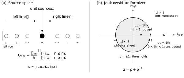
The source row splices the left solution $\ell$ to the remote solution $r$. For the free Jacobi chain, $z=\rho+\rho^{-1}$ separates the physical sheet $|\rho|<1$ from its continuation: $\rho_*=1/h$ is a bound-state pole for $|h|>1$, an antibound pole for $0<|h|<1$, and a threshold at $|h|=1$. The markers are shown for $h>0$; negative $h$ reflects them through the origin.

Recurrence data reach the ODE through a transfer theorem

The coefficient Green matrix is not automatically the Green kernel of the differential equation that generated the recurrence. Let an adapted expansion be written schematically as

$$y(z,\lambda) = \mathcal S(\lambda)u = \sum_{n=0}^{\infty} u_n(\lambda)\,\phi_n(z,\lambda),$$

where the prefactor, gauge, basis functions, branch choices, and convergence domain are all part of the synthesis map $\mathcal S$. An ODE source also has to be converted to a coefficient source by some map $\mathcal Q$. Only after those maps have been constructed does one obtain a relation of the form

$$\mathcal G_{\mathrm{ODE}}(\lambda) = \mathcal S(\lambda) T(\lambda)^{-1} \mathcal Q(\lambda).$$

Locally near a candidate pole, a useful sufficient transfer ledger is:

1. The adapted series represents the normalized left ODE solution on a declared branch.

2. The exact remote recurrence line represents the normalized right ODE condition. This requires the large-order transfer theorem developed on the connection-amplitude page, not merely a stable finite cutoff.

3. The series, recurrence tail, and required parameter derivatives converge locally uniformly.

4. Exceptional recurrence indices and any gauge zeros or poles have been handled homogeneously.

5. The ODE boundary Wronskian and recurrence denominator obey

   $$D_{\mathrm{ODE}}(\lambda) = C(\lambda)\Delta(\lambda), \qquad C(\lambda_*)\neq0,$$

   on the same analytic sheet.

6. The synthesis and source maps are analytic at $\lambda_*$ and do not annihilate the residue.

The nonzero conversion factor $C$ preserves zeros and multiplicities, but not derivative normalizations:

$$D_{\mathrm{ODE}}'(\lambda_*) = C(\lambda_*)\Delta'(\lambda_*).$$

Therefore $1/\Delta'(\lambda_*)$ is not a physical excitation factor until the endpoint normalizations and the conversion factor have been retained.

QNM conditions are convention-locked intersections

Consider, only as a local model for the signs, the radial equation

$$\mathscr L_\omega u = \frac{\dd^2u}{\dd x^2} +\left[ \omega^2-V(x) \right]u =0$$

with time dependence $\ee^{-\ii\omega t}$. Let

$$\begin{aligned} f_L(x,\omega) &\sim \ee^{-\ii\omega x}, &&x\to-\infty, \\ f_R(x,\omega) &\sim \ee^{+\ii\omega x}, &&x\to+\infty. \end{aligned}$$

In a black-hole interpretation these are, respectively, future-horizon ingoing and spatial-infinity outgoing for the stated Fourier convention. The detailed endpoint conditions—and their changes in rotating, charged, de Sitter, or anti-de Sitter problems—are recorded on the spectral boundary page.

If

$$f_L = A_{\mathrm{out}}f_R +A_{\mathrm{in}}f_{\mathrm{in}}$$

at the right endpoint, with $f_{\mathrm{in}}\sim\ee^{-\ii\omega x}$, then the chapter’s Wronskian orientation gives

$$\Wr[f_L,f_R] = 2\ii\omega A_{\mathrm{in}}.$$

The Green kernel solving $\mathscr L_\omega\widetilde G(\,\cdot\,,y;\omega) =\delta(\,\cdot\!-y)$ is

$$\widetilde G(x,y;\omega) = \frac{ f_L(x_<,\omega)f_R(x_>,\omega) }{ \Wr[f_L,f_R](\omega) },$$

where

$$x_<=\min(x,y), \qquad x_>=\max(x,y).$$

For a simple zero $\omega_q\neq0$ of $A_{\mathrm{in}}$,

$$\underset{\omega=\omega_q}{\operatorname{Res}} \,\widetilde G = \frac{ f_L(x_<,\omega_q)f_R(x_>,\omega_q) }{ 2\ii\omega_q A_{\mathrm{in}}'(\omega_q) }.$$

For a stable causal problem, the retarded transform is initially holomorphic in the upper half-plane; more generally its first domain is a half-plane fixed by the causal growth bound. With $\ee^{-\ii\omega t}$, damped QNMs lie in $\operatorname{Im}\omega<0$. Reversing the Fourier convention reverses the printed radiation phases and the damping half-plane.

A recurrence residual becomes this QNM denominator only if the transfer ledger proves, on the chosen sheet,

$$\Wr[f_L,f_R](\omega) = C(\omega)\Delta(\omega), \qquad C(\omega_q)\neq0.$$

Minimality in coefficient index is not synonymous with spatial decay. For decaying QNMs the physical radial function often grows exponentially at both ends of a real tortoise-coordinate contour; the minimal coefficient line represents an analytically continued outgoing condition, not an $L^2$ state.

The QNM implication

A zero of $\Delta(\omega)$ proves that two selected recurrence lines intersect. It is a QNM only after those lines have been proved to represent the two physical boundary conditions and after a resolvent- or generator-based pole theorem has been supplied for the problem at hand.

A hypergeometric QNM control experiment

The Pöschl–Teller barrier provides an exact audit of the entire transfer chain. It is not a generic three-term continued-fraction problem—its Taylor recurrence degenerates to two terms—but precisely for that reason every normalization can be checked in closed form. This complements the earlier hypergeometric connection benchmark, where the same connection technology was audited without radiation conditions.

Let

$$V(x) = V_0\operatorname{sech}^2(\alpha x), \qquad V_0>0, \quad \alpha>0,$$

and set

$$\begin{aligned} \zeta &= \frac{1+\tanh(\alpha x)}2, \\ \nu &= \sqrt{ \frac{V_0}{\alpha^2}-\frac14 }, \\ q &= -\frac{\ii\omega}{2\alpha}. \end{aligned}$$

Choose a branch of $\nu$ once and for all. A left-ingoing solution is

$$f_L = \zeta^q(1-\zeta)^q {}_2F_1(a,b;c;\zeta),$$

where

$$\begin{aligned} a &= \frac12-\frac{\ii\omega}{\alpha}+\ii\nu, \\ b &= \frac12-\frac{\ii\omega}{\alpha}-\ii\nu, \\ c &= 1-\frac{\ii\omega}{\alpha}. \end{aligned}$$

The Taylor coefficients

$${}_2F_1(a,b;c;\zeta) = \sum_{k=0}^{\infty}d_k\zeta^k, \qquad d_0=1,$$

obey the exact recurrence

$$(k+1)(k+c)d_{k+1} = (k+a)(k+b)d_k.$$

The connection formula at $\zeta=1$ yields

$$\begin{aligned} A_{\mathrm{in}} &= \frac{ \Gamma(c)\Gamma(-\ii\omega/\alpha) }{ \Gamma(a)\Gamma(b) }, \\ A_{\mathrm{out}} &= \frac{ \Gamma(c)\Gamma(\ii\omega/\alpha) }{ \Gamma(c-a)\Gamma(c-b) }. \end{aligned}$$

Thus

$$\Wr[f_L,f_R] = 2\ii\omega A_{\mathrm{in}},$$

and, away from exceptional gamma-function cancellations, the QNM frequencies are

$$\omega_n^\pm = \alpha \left[ \pm\nu-\ii\left(n+\frac12\right) \right], \qquad n=0,1,2,\ldots.$$

For the plus ladder, $a=-n$; for the minus ladder, $b=-n$. At generic parameters, with the recurrence denominator nonzero at the closing step, the coefficient recurrence terminates at the same parameter. Exceptional numerator–denominator coincidences must instead be evaluated through an analytic limit of the hypergeometric solution. Termination is spectral here not because every polynomial is a QNM, but because the prefactors and the independent gamma-function connection formula prove both radiation conditions.

For example,

$$\alpha=1, \qquad V_0=\frac54, \qquad \nu=1, \qquad n=1$$

gives

$$\begin{gathered} \omega_1^+ = 1-\frac32\ii, \\ a=-1, \qquad b=-1-2\ii, \\ c=-\frac12-\ii. \end{gathered}$$

and

$$d_0=1, \qquad d_1=-2, \qquad d_2=0.$$

This is a compact exact unit test: the recurrence terminates, the incoming connection coefficient vanishes, and the Wronskian pole condition agrees without fitting any conversion factor.

At $\nu=0$ the two ladders coalesce. Here $a=b=-n$ while the numerator gamma factors remain finite, so $A_{\mathrm{in}}$ has a double zero. Checking the analytic Green numerator confirms a second-order operator pole in this model, although a specially projected matrix element may still cancel. In a general problem, coincident frequency lists do not replace the geometric-multiplicity and local-Laurent tests for an exceptional point.

Poles can disappear from a measured entry

An operator pole need not appear in every matrix element. Suppose the coefficient inverse is inserted into a scalar source-to-observable map,

$$\mathcal M(\lambda) = L(\lambda)\, \mathcal S(\lambda)\, T(\lambda)^{-1}\, \mathcal Q(\lambda).$$

At a simple characteristic value, the Keldysh formula gives

$$\underset{\lambda=\lambda_*}{\operatorname{Res}} \,\mathcal M = \frac{ \bigl(L\mathcal S v\bigr) \bigl(w^*\mathcal Q\bigr) }{ w^*T'v }.$$

The full inverse has a pole, but the measured scalar does not if the observable annihilates the right mode or the source is orthogonal to the left mode. A zero numerator is a selection rule or cancellation, not proof that the underlying mode is absent.

The same point appears in a boundary response ratio. If

$$u_{\mathrm{in}} = A(\omega)u_{\mathrm{src}} +B(\omega)u_{\mathrm{resp}},$$

then a retarded response often has the schematic form

$$G_{\mathrm R}(\omega) = \mathcal N(\omega) \frac{B(\omega)}{A(\omega)} +P(\omega),$$

where $P$ is analytic contact-term data. A zero of $A$ gives a response pole only if $B$ and $\mathcal N$ do not cancel it. If locally

$$A\sim a_p(\omega-\omega_*)^p, \qquad B\sim b_q(\omega-\omega_*)^q,$$

then $B/A$ has pole order $\max(p-q,0)$. The fully normalized holographic interpretation belongs to Chapter 15; the algebraic numerator audit already belongs here.

Branch points and multiple roots need separate diagnoses

The statement “the denominator vanishes” does not classify the singularity.

Threshold coalescence

At $\omega=0$,

$$\Wr[ \ee^{-\ii\omega x}, \ee^{+\ii\omega x} ] = 2\ii\omega$$

vanishes because the two radiation labels coalesce. This is a degeneration of the chosen basis, not automatically a zero-frequency mode. One should uniformize the threshold, as the $\rho$ coordinate did for the Jacobi chain, before assigning a pole order.

Branch cuts

The right recurrence solution can be multivalued in the spectral parameter. Long-range wave problems, massive thresholds, and extremal limits commonly produce branch points. A root search must record the sheet and the lateral value of any cut. A QNM residue sum then need not be a complete time-domain representation; cut integrals and large-frequency arcs can contribute prompt signals and late-time tails.

Exceptional points

A double zero of one scalar characteristic function is not, by itself, an exceptional point. The possibilities include:

• a semisimple degeneracy with two eigenvectors and a rank-two simple resolvent pole;
• a defective eigenvalue with a Jordan chain and a higher-order pole;
• a scalar numerator that reduces the pole order;
• a threshold branch singularity rather than a meromorphic pole.

For a defective order-two point, the inverse transform contains a term proportional to

$$t\,\ee^{-\ii\omega_*t}.$$

The geometric multiplicity and local Laurent expansion—not only $\Delta=\Delta'=0$—make the classification.

Separated QNM problems can remain coupled

In Kerr-type problems the angular separation constant $A$ is not an arbitrary external parameter. The physical mode solves

$$\begin{aligned} F_{\mathrm{ang}}(A,\omega)&=0,\\ F_{\mathrm{rad}}(A,\omega)&=0. \end{aligned}$$

A radial continued-fraction root at an unrelated fixed value of $A$ is not a Kerr QNM. If $F_{\mathrm{ang},A}\neq0$, the implicit-function theorem gives

$$A'(\omega) = - \frac{ F_{\mathrm{ang},\omega} }{ F_{\mathrm{ang},A} }.$$

Along the angular eigenvalue branch,

$$\begin{aligned} \frac{\dd}{\dd\omega} F_{\mathrm{rad}}\bigl(A(\omega),\omega\bigr) &= F_{\mathrm{rad},\omega} +A'(\omega)F_{\mathrm{rad},A} \\ &= F_{\mathrm{rad},\omega} - F_{\mathrm{rad},A} \frac{ F_{\mathrm{ang},\omega} }{ F_{\mathrm{ang},A} }. \end{aligned}$$

Using only the radial partial derivative gives the wrong residue and the wrong root condition number. At a genuinely coupled simple root, nonvanishing of the Jacobian determinant of $(F_{\mathrm{ang}},F_{\mathrm{rad}})$ with respect to $(A,\omega)$ is the invariant local test.

A recurrence-to-pole audit

Before reporting a recurrence zero as a pole or QNM, record the following.

Datum	Required check
Recurrence	All ordinary and exceptional rows, including any reduction from a higher-term relation
Left line	The precise local ODE condition represented by the endpoint row
Right line	A theorem identifying the exact minimal tail with the remote physical or continued condition
Characteristic function	A homogeneous Casoratian form that survives ratio-chart failures
Parameter dependence	Local holomorphy or a declared branch and locally uniform convergence
Spectral variable	Whether the analytic coordinate is $\lambda$, $k$, $\omega$, $\omega^2$, or a uniformizer
Operator meaning	Space, domain, Fredholm family, and physical or continued resolvent
Coupled constraints	Angular, gauge, constraint, or interface conditions solved simultaneously
Residue	Left–right derivative pairing plus all conversion and normalization factors
Numerator	Source and observable couplings that may remove an entry pole
Independent check	Direct Wronskian matching, integration, or an exactly solvable connection formula

The next page turns the last line into a numerical protocol: cutoff studies, precision escalation, condition estimates, residuals, and independent representations.

Common pitfalls

Calling a formal sequence kernel physical. The splice formula solves an inhomogeneous recurrence. A sequence-to-ODE transfer theorem and an operator or continuation construction are still required before it becomes a physical Green function.

Forgetting the source weight. For a nonsymmetric recurrence the Green matrix contains $\varpi_m$ and is not ordinarily symmetric. Omitting that factor preserves some zero locations but corrupts source amplitudes and residues.

Differentiating an arbitrary residual normalization. Multiplying a characteristic function by a nonzero analytic factor preserves its roots but rescales its derivative. A physical residue requires the numerator and the conversion factor to be normalized consistently.

Equating minimal with square summable. On a continued QNM sheet the minimal coefficient sequence can reconstruct a spatially growing outgoing wave. Minimality is relative to another sequence solution, not a universal Hilbert-space condition.

Ignoring a ratio-chart pole. A zero of $r_0$ makes $r_1/r_0$ undefined. The homogeneous Casoratian residual remains the correct line-intersection test.

Calling every double root exceptional. Zero order, geometric multiplicity, Laurent pole order, and residue rank are distinct. A Jordan chain or equivalent local resolvent evidence is needed.

Searching without a sheet ledger. A bound state, antibound state, threshold, and resonance can share one algebraic equation in a uniformizing coordinate. Their sheet and endpoint condition make them different objects.

Solving only half of a separated problem. In rotating problems the angular and radial characteristic equations are coupled through the separation constant. Holding it arbitrarily fixed changes the spectral problem.

Exercises

1. Derive the sequence Green matrix

Starting from the proposed splice formula, verify every homogeneous row, the left endpoint row, and the source jump. Then prove that

$$\Delta = \varpi_n\alpha_n\mathcal K_n$$

is independent of $n$ and derive the weighted reciprocity relation.

Solution

For fixed $m$ and $n<m$, the Green column is

$$G_{nm} = \frac{ \varpi_mr_m }{ \Delta }\ell_n,$$

so it satisfies the homogeneous recurrence, including the left row when $m>0$. For $n>m$ it is

$$G_{nm} = \frac{ \varpi_m\ell_m }{ \Delta }r_n,$$

and therefore obeys the chosen right condition. For $m\geq1$, the source row is

$$\begin{aligned} \bigl(TG_{\bullet m}\bigr)_m &= \frac{\varpi_m}{\Delta} \left[ \alpha_m\ell_mr_{m+1} +\beta_m\ell_mr_m +\gamma_m\ell_{m-1}r_m \right] \\ &= \frac{ \varpi_m\alpha_m\mathcal K_m }{ \Delta } =1. \end{aligned}$$

When $m=0$, use the endpoint row separately:

$$\begin{aligned} \bigl(TG_{\bullet0}\bigr)_0 &= \frac{ \ell_0 \left( \alpha_0r_1+\beta_0r_0 \right) }{ \alpha_0\mathcal K_0 } \\ &= 1, \end{aligned}$$

where the last equality follows from $\beta_0\ell_0=-\alpha_0\ell_1$.

For $n\geq1$, the discrete Abel identity gives

$$\alpha_n\mathcal K_n = \gamma_n\mathcal K_{n-1}.$$

Since

$$\varpi_n\gamma_n = \varpi_{n-1}\alpha_{n-1},$$

one obtains

$$\varpi_n\alpha_n\mathcal K_n = \varpi_{n-1}\alpha_{n-1}\mathcal K_{n-1}.$$

Finally,

$$\begin{aligned} \varpi_nG_{nm} &= \frac{ \varpi_n\varpi_m \ell_{\min(n,m)}r_{\max(n,m)} }{ \Delta } \\ &= \varpi_mG_{mn}. \end{aligned}$$

2. Recover the finite cofactor identity

Let $T_N$ be the tridiagonal block on $0,\ldots,N$, let $D_N=\det T_N$, and let $E_1^{[N]}$ be the determinant of the trailing block on $1,\ldots,N$. Prove

$$\left(T_N^{-1}\right)_{00} = \frac{E_1^{[N]}}{D_N} = \frac1{F_0^{[N]}}.$$

What remains true when $E_1^{[N]}=0$?

Solution

The $(0,0)$ cofactor of $T_N$ is exactly $E_1^{[N]}$. Cramer’s rule therefore gives

$$\left(T_N^{-1}\right)_{00} = \frac{E_1^{[N]}}{D_N}$$

whenever $D_N\neq0$. The trailing-continuant calculation on the preceding page gives

$$F_0^{[N]} = \frac{D_N}{E_1^{[N]}}$$

when the ratio chart is valid, proving the reciprocal identity.

If $E_1^{[N]}=0$, the displayed continued fraction has a chart pole. Cramer’s cofactor formula and the cross-multiplied continuant identity remain valid. In particular, a simultaneous analysis of $D_N$ and $E_1^{[N]}$ is needed; one must not infer a spectral point from the divergent affine fraction alone.

3. Audit the Jacobi chain with a boundary impurity

Derive the left solution

$$\ell_n = U_n(z/2)-hU_{n-1}(z/2),$$

the full Green kernel, the pole classification, and the residue

$$\underset{z=z_*}{\operatorname{Res}} \,G_{nm} = - \left(1-h^{-2}\right)h^{-(n+m)}$$

for real $|h|>1$.

Solution

The Chebyshev recurrence

$$U_{n+1}(z/2) = zU_n(z/2)-U_{n-1}(z/2)$$

shows that $\ell$ satisfies the interior equation. Since $U_{-1}=0$, $U_0=1$, and $U_1=z$,

$$\ell_0=1, \qquad \ell_1=z-h,$$

which is the left row of $(J_h-zI)\ell=0$.

With $r_n=\rho^n$ and $z=\rho+\rho^{-1}$,

$$\Delta = \ell_0r_1-\ell_1r_0 = h-\rho^{-1}.$$

The splice theorem gives

$$G_{nm} = \frac{ \ell_{\min(n,m)} \rho^{\max(n,m)} }{ h-\rho^{-1} }.$$

The zero occurs at $\rho_*=h^{-1}$. It is inside the physical disk for $|h|>1$, outside it for $0<|h|<1$, and at a branch point for $|h|=1$.

Differentiate the uniformization:

$$\frac{\dd z}{\dd\rho} = 1-\rho^{-2}.$$

Since

$$\frac{\dd\Delta}{\dd\rho} = \rho^{-2},$$

one finds

$$\Delta'(z_*) = \frac1{\rho_*^2-1}.$$

At the pole, $\ell_n=r_n=\rho_*^n$. Hence

$$\begin{aligned} \underset{z=z_*}{\operatorname{Res}} \,G_{nm} &= \frac{ \rho_*^{n+m} }{ \Delta'(z_*) } \\ &= - \left(1-\rho_*^2\right) \rho_*^{n+m}, \end{aligned}$$

which becomes the stated formula after $\rho_*=h^{-1}$.

4. Derive a simple pencil residue and a cancellation

Assume the right and left nullspaces of $T(\lambda_*)$ are one-dimensional. Let $T(\lambda_*)v=0$ and $w^*T(\lambda_*)=0$, with $w^*T'(\lambda_*)v\neq0$. Derive the rank-one Laurent coefficient. Then give a $2\times2$ example in which the inverse has a pole but one diagonal entry does not.

Solution

For a source $f$, write the singular part of the solution as

$$u(\lambda) = \frac{a(f)}{\lambda-\lambda_*}v+O(1).$$

Insert this into $T(\lambda)u=f$ and use

$$T(\lambda) = T(\lambda_*) +(\lambda-\lambda_*)T'(\lambda_*) +O\left((\lambda-\lambda_*)^2\right).$$

The constant-order equation, projected with $w^*$, is

$$a(f)\,w^*T'(\lambda_*)v = w^*f.$$

Therefore

$$a(f) = \frac{w^*f}{w^*T'(\lambda_*)v},$$

and

$$\underset{\lambda=\lambda_*}{\operatorname{Res}} \,T(\lambda)^{-1} = \frac{v\,w^*}{w^*T'(\lambda_*)v}.$$

For a cancellation, take

$$T(\lambda) = \begin{pmatrix} \lambda&0\\ 0&1 \end{pmatrix}.$$

Then

$$T(\lambda)^{-1} = \begin{pmatrix} \lambda^{-1}&0\\ 0&1 \end{pmatrix}.$$

The inverse operator has a pole at zero, but its $(2,2)$ entry does not. The source and observable associated with the second coordinate annihilate the singular eigenprojection.

5. Verify the Pöschl–Teller mode condition

Starting from the hypergeometric connection formula, verify

$$A_{\mathrm{in}} = \frac{ \Gamma(c)\Gamma(-\ii\omega/\alpha) }{ \Gamma(a)\Gamma(b) }$$

and derive the two QNM ladders. For the plus ladder, explain why the Taylor series terminates.

Solution

The connection formula separates a term analytic at $\zeta=1$ from a term multiplied by

$$(1-\zeta)^{c-a-b}.$$

Here

$$c-a-b = \frac{\ii\omega}{\alpha}.$$

The common prefactor contributes $(1-\zeta)^{-\ii\omega/(2\alpha)}$. Since $1-\zeta\sim\ee^{-2\alpha x}$, the analytic term is proportional to $\ee^{+\ii\omega x}$ and the second term to $\ee^{-\ii\omega x}$. The coefficient of the latter is

$$A_{\mathrm{in}} = \frac{ \Gamma(c)\Gamma(a+b-c) }{ \Gamma(a)\Gamma(b) } = \frac{ \Gamma(c)\Gamma(-\ii\omega/\alpha) }{ \Gamma(a)\Gamma(b) }.$$

The gamma function has no zeros. Away from exceptional coincidences, $A_{\mathrm{in}}=0$ when either denominator gamma function has a pole:

$$a=-n \quad\text{or}\quad b=-n.$$

Solving these equations gives

$$\omega_n^\pm = \alpha \left[ \pm\nu-\ii\left(n+\frac12\right) \right].$$

On the plus ladder, $a=-n$. Provided $(n+1)(n+c)\neq0$ and no later denominator collision occurs, the coefficient recurrence contains the factor $k+a$, so at $k=n$ it gives $d_{n+1}=0$; all later coefficients vanish. At an exceptional collision, the same statement has to be read through the analytic hypergeometric limit. The polynomial alone does not prove the QNM condition—the connection coefficient supplies that proof.

6. Differentiate a coupled angular–radial condition

Assume

$$F_{\mathrm{ang}}(A,\omega)=0, \qquad F_{\mathrm{ang},A}\neq0.$$

Derive $A'(\omega)$ and the total derivative of $F_{\mathrm{rad}}(A(\omega),\omega)$. Express the condition for an isolated coupled root as a Jacobian.

Solution

Implicit differentiation gives

$$F_{\mathrm{ang},A}A' +F_{\mathrm{ang},\omega} =0,$$

so

$$A' = - \frac{ F_{\mathrm{ang},\omega} }{ F_{\mathrm{ang},A} }.$$

The chain rule then yields

$$\frac{\dd F_{\mathrm{rad}}}{\dd\omega} = F_{\mathrm{rad},\omega} - F_{\mathrm{rad},A} \frac{ F_{\mathrm{ang},\omega} }{ F_{\mathrm{ang},A} }.$$

The coupled root is locally isolated when

$$\det \begin{pmatrix} F_{\mathrm{ang},A} & F_{\mathrm{ang},\omega} \\ F_{\mathrm{rad},A} & F_{\mathrm{rad},\omega} \end{pmatrix} \neq0.$$

Multiplying the total radial derivative by $F_{\mathrm{ang},A}$ recovers this determinant exactly.

7. Distinguish an exceptional point from a degeneracy

Compare

$$T_{\mathrm{EP}}(\lambda) = \begin{pmatrix} \lambda&-1\\ 0&\lambda \end{pmatrix}$$

with $T_{\mathrm{ss}}(\lambda)=\lambda I_2$. Determine the kernel dimensions and pole orders of the inverses.

Solution

Direct inversion gives

$$T_{\mathrm{EP}}(\lambda)^{-1} = \begin{pmatrix} \lambda^{-1}&\lambda^{-2}\\ 0&\lambda^{-1} \end{pmatrix}.$$

At $\lambda=0$, the kernel is one-dimensional and the $\lambda^{-2}$ term records a length-two Jordan chain. This is a defective exceptional point.

By contrast,

$$T_{\mathrm{ss}}(\lambda)^{-1} = \lambda^{-1}I_2.$$

Its kernel at zero is two-dimensional and the inverse has only a simple pole, now with rank-two residue. Both determinants vanish to order two, showing that determinant order alone distinguishes neither geometric multiplicity nor resolvent pole order.

References

• NIST Digital Library of Mathematical Functions, §15.8, “Transformations of Variable”, for the hypergeometric connection formulas used in the Pöschl–Teller audit.
• G. Teschl, Jacobi Operators and Completely Integrable Nonlinear Lattices, equations (1.20)–(1.21) and (1.95)–(1.99), for the discrete Lagrange identity, conserved Wronskian, and Jacobi Green kernel.
• F. Gesztesy and B. Simon, “$m$-Functions and Inverse Spectral Analysis for Finite and Semi-Infinite Jacobi Matrices”, Journal d’Analyse Mathématique 73 (1997), 267–297, for half-line Jacobi resolvents and Weyl functions.
• D. Damanik and B. Simon, “Jost Functions and Jost Solutions for Jacobi Matrices, I”, Inventiones Mathematicae 165 (2006), 1–50, for Joukowski uniformization and Jacobi Jost analyticity.
• S. Güttel and F. Tisseur, “The Nonlinear Eigenvalue Problem”, Acta Numerica 26 (2017), 1–94, for Keldysh expansions, left–right normalization, conditioning, and multiple eigenvalues.
• E. W. Leaver, “An Analytic Representation for the Quasi-Normal Modes of Kerr Black Holes”, Proceedings of the Royal Society A 402 (1985), 285–298, for the minimal recurrence and coupled continued-fraction QNM construction.
• E. W. Leaver, “Spectral Decomposition of the Perturbation Response of the Schwarzschild Geometry”, Physical Review D 34 (1986), 384–408, for Green-function poles, QNM residues, branch-cut contributions, and prompt response.
• H.-P. Nollert and B. G. Schmidt, “Quasinormal Modes of Schwarzschild Black Holes: Defined and Calculated via Laplace Transformation”, Physical Review D 45 (1992), 2617–2627, for the causal Green-function definition and continued-fraction computation.
• E. Berti and V. Cardoso, “Quasinormal Ringing of Kerr Black Holes: The Excitation Factors”, Physical Review D 74 (2006), 104020, for Wronskian derivatives, source-independent excitation factors, and the Pöschl–Teller audit.
• S. Dyatlov, “Quasi-Normal Modes and Exponential Energy Decay for the Kerr–de Sitter Black Hole”, Communications in Mathematical Physics 306 (2011), 119–163, for QNMs as poles of a meromorphic operator family.
• C. M. Warnick, “On Quasinormal Modes of Asymptotically Anti-de Sitter Black Holes”, Communications in Mathematical Physics 333 (2015), 959–1035, for the generator framework, boundary conditions, and limitations of mode completeness.
• M. Casals and A. C. Ottewill, “Analytic Investigation of the Branch Cut of the Green Function in Schwarzschild Space-Time”, Physical Review D 87 (2013), 064010, for sheet-dependent cut contributions and their relation to QNM structure.

Next page

The verified-numerics capstone turns these exact identities into a computational protocol: stable recurrence direction, tail enclosures, precision selection, residual and derivative conditioning, root counts, and checks against an independent ODE representation.