Decoupling Limits, Irregular Punctures, and Confluent Equations

An asymptotically free limit is not obtained by merely setting the four-puncture cross-ratio to zero. One mass must diverge while the cross-ratio vanishes, and their product must retain a dimensionful renormalization-group scale. On the gauge side this operation removes a hypermultiplet from every fixed-point coefficient. On the CFT side two regular punctures collide while their momenta diverge, leaving an irregular state rather than an ordinary primary. After a degenerate probe and the NS limit are added, the four-regular-singularity oper becomes a confluent-Heun oper.

This page carries out that chain for $SU(2)$ with $N_f=4\to3$ in the exact matter convention fixed on the regular-puncture page. The calculation exposes two pieces that are often lost in a schematic collision: the equivariant centering of the heavy mass and the finite exponential inherited from the Heisenberg factor. It then follows the remaining flavor decouplings far enough to show why they do not form a one-to-one copy of the standard named Heun hierarchy.

First pass

Read the fixed-point limit, the irregular-state passport, and the two-ladder diagram. The normal-form accessory remainder is the precision check needed when an actual confluent-Heun coefficient must be computed.

Status ledger

Statement used on this page	Status
Fixed-diagram $N_f=4\to3$ instanton limit	Exact coefficientwise algebra for the declared box factors, at generic parameters away from localization poles
Decoupling of the full classical and one-loop partition function	Scheme-dependent until heavy-hypermultiplet counterterms and local factors are fixed; not asserted here
Regular block $\to$ rank-one irregular block	Formal, order-by-order collision of chiral blocks after a divergent scalar normalization is chosen
Inherited $N_f=3$ AGT equality	Formal-series identity in the declared collision and Heisenberg normalization
Irregular Virasoro constraints and finite-$b$ confluent BPZ equation	Exact after the irregular-state and null-vector normalizations are fixed
Degenerate insertion $\leftrightarrow$ gauge surface defect	Proposed and evidence-supported in specific AGT constructions, not a universal theorem; the next page states the realization data
Heavy or NS reduction of BPZ to an oper	Conditional on derivative-compatible factorization along the declared centered-mass path
Normal-form confluence and $u=-\lim A(c_A+mL)$	Exact coefficient algebra and locally uniform outer limit once the printed scaling is imposed
Identification of $u$ with an NS scale derivative	Convention-dependent: leading scale power, Heisenberg factor, contacts, logarithm branch, and fixed variables must be specified
Generic CHE scalar-gauge dictionary	Exact for $L\neq0$ on a chosen branch; local resonances require separate basis conventions
Universal rule “$N_f=n$ equals the $n$th named Heun confluence”	False; puncture realization, ramification, coordinate cover, and scalar gauge must also be given

Decoupling is a scaled collision, not an ordinary cusp

Keep the four-puncture placement $(\infty,1,t,0)$ and the printed matter orientation from the preceding page: $\mu_{1,2}$ are antifundamental Nekrasov masses and $\mu_{3,4}$ are fundamental masses. Center every printed mass by

$$M_i = \mu_i-\frac{\epsilon_\Sigma}{2}, \qquad i=1,2,3,4.$$

Only $M_3$ and $M_4$ enter the first collision; $M_1$ and $M_2$ become useful in the reverse CHE map.

The first decoupling limit is

$$\begin{gathered} t\longrightarrow0, \qquad M_4\longrightarrow\infty, \qquad \mathfrak q_3:=-\lim t\mu_4=-\lim tM_4, \\ a_{\mathrm C},\ \mu_1,\ \mu_2,\ M_3, \ \epsilon_1,\ \epsilon_2 \quad\text{fixed}. \end{gathered}$$

The two definitions of $\mathfrak q_3$ have the same limit because $t(\mu_4-M_4)=t\epsilon_\Sigma/2\to0$. They should nevertheless not be identified at finite $t$. The printed mass is natural in the localization box factor; the centered mass gives the clean collision of Liouville momenta and oper exponents. This finite-$t$ distinction will matter when a subleading accessory remainder is extracted.

The mass dimension already diagnoses the physics. The four-flavor fugacity $t$ is dimensionless, while

$$[\mathfrak q_3]=1.$$

More generally, if $\mathfrak q_n$ denotes the instanton coordinate for the $N_f=n$ theory, then

$$[\mathfrak q_n]=4-n, \qquad \mathfrak q_n=c_n\Lambda_n^{4-n}.$$

The nonzero constant $c_n$ is a scale convention. Sending a printed fundamental mass to infinity gives $\mathfrak q_{n-1}=-\mu_{\mathrm f}\mathfrak q_n$ in the present box convention; sending a printed antifundamental mass to infinity gives $\mathfrak q_{n-1}=+\mu_{\mathrm{af}}\mathfrak q_n$. A sign or root absorbed into $\Lambda_n$ is therefore part of the passport, not a universal fact.

For example, removing the printed masses in the order $\mu_4,\mu_3,\mu_2,\mu_1$ gives the oriented formal scale chain

$$\begin{aligned} \mathfrak q_4&=t, & \mathfrak q_3&=-t\mu_4, \\ \mathfrak q_2&=+t\mu_3\mu_4, & \mathfrak q_1&=+t\mu_2\mu_3\mu_4, \\ \mathfrak q_0&=+t\mu_1\mu_2\mu_3\mu_4. \end{aligned}$$

This display fixes only the fixed-point fugacities. Converting them to Seiberg–Witten scales or distributing their powers between two irregular states may introduce finite constants and branch choices.

If instead $t\to0$ with every mass fixed, the theory simply approaches the weak-coupling cusp of the conformal $N_f=4$ theory. Its instanton series tends to $1$, its two colliding punctures retain finite momenta, and no finite irregular moment survives. The same small coordinate thus describes two different limits:

Limit near $t=0$	Data held fixed	Result
Ordinary cusp	All four masses	Weakly coupled $N_f=4$ theory and a regular OPE degeneration
Flavor decoupling	$\mathfrak q_3=-t\mu_4$ and the three light masses	Asymptotically free $N_f=3$ theory and an irregular collision

Every Young-diagram coefficient has a finite three-flavor limit

For a box $s=(i,j)$ in the diagram $Y_\alpha$, recall

$$\phi(a_\alpha,s) = a_\alpha+\epsilon_1(i-1)+\epsilon_2(j-1).$$

The printed fundamental factor of the heavy fourth flavor is

$$z_{\mathrm{fund}}(\boldsymbol a,\boldsymbol Y;\mu_4) = \prod_{\alpha=1}^{2} \prod_{s\in Y_\alpha} \left[ \phi(a_\alpha,s)-\mu_4+\epsilon_\Sigma \right].$$

At a fixed pair of diagrams $\boldsymbol Y=(Y_1,Y_2)$ with $k=|\boldsymbol Y|$ boxes,

$$z_{\mathrm{fund}}(\boldsymbol a,\boldsymbol Y;\mu_4) = (-\mu_4)^k \left[1+O(\mu_4^{-1})\right].$$

Consequently,

$$t^k z_{\mathrm{fund}}(\boldsymbol a,\boldsymbol Y;\mu_4) \longrightarrow \mathfrak q_3^k.$$

All vector and light-matter factors remain unchanged. Therefore, for generic equivariant parameters and away from their meromorphic poles, the limit exists coefficient by coefficient:

$$\begin{aligned} Z_{\mathrm{inst}}^{U(2),N_f=4} \left(a_{\mathrm C},\boldsymbol\mu;t\right) \longrightarrow Z_{\mathrm{inst}}^{U(2),N_f=3} \left( a_{\mathrm C}; \mu_1,\mu_2,\mu_3; \mathfrak q_3 \right). \end{aligned}$$

This is a statement about normalized formal instanton series. At each power of $\mathfrak q_3$ there are finitely many diagram pairs, so the termwise argument is sufficient. Interchanging this limit with an infinite sum, analytically continuing through poles, or integrating over $a_{\mathrm C}$ requires additional uniformity or contour data.

The one-box coefficient from the regular page gives a fast independent audit. Let $P_\pm^{(3)}$ be its polynomials $P_\pm$ with the fourth fundamental factor deleted, and set

$$Z_1^{(3)} = -\frac{1}{\epsilon_1\epsilon_2} \left[ \frac{P_+^{(3)}}{2a_{\mathrm C}(2a_{\mathrm C}+\epsilon_\Sigma)} + \frac{P_-^{(3)}}{2a_{\mathrm C}(2a_{\mathrm C}-\epsilon_\Sigma)} \right].$$

Both deleted factors are $-\mu_4+O(1)$, so

$$tZ_1^{(4)} \longrightarrow \mathfrak q_3Z_1^{(3)}.$$

The two colored-box terms are still exchanged by $a_{\mathrm C}\mapsto-a_{\mathrm C}$, and $[\mathfrak q_3Z_1^{(3)}]=0$. One line therefore checks the sign, dimension, and Weyl symmetry of the limit.

The sign in $\mathfrak q_3=-t\mu_4$ is not optional in this representative: it comes from the leading $-\mu_4$ of every fundamental box. Reflecting that flavor into an antifundamental changes both the printed mass and the sign rule. This elementary box audit is safer than importing a scale matching formula from a different matter orientation.

Divergent centered masses leave finite Virasoro moments

The regular mass passport reads

$$p_t=\frac{M_3+M_4}{2}, \qquad p_0=\frac{M_3-M_4}{2}.$$

Thus the two momenta that collide at $0$ do not stay finite. On the centered collision path

$$M_4=-\frac{\mathfrak q_3}{t},$$

they behave as

$$\begin{aligned} p_t &= -\frac{\mathfrak q_3}{2t}+\frac{M_3}{2}, & p_0 &= +\frac{\mathfrak q_3}{2t}+\frac{M_3}{2}. \end{aligned}$$

The divergent parts are equal and opposite. They cancel in $p_t+p_0=M_3$ but survive in the scaled moments of the collision. This is precisely what distinguishes an irregular state from the highest- weight state obtained by an ordinary OPE limit.

Define dimensionless irregular parameters

$$R = \frac{M_4}{\varepsilon_\star}, \qquad \Lambda_{\mathcal I} = \frac{tM_4}{\varepsilon_\star} = -\frac{\mathfrak q_3}{\varepsilon_\star}, \qquad \mu_{\mathcal I} = -\frac{M_3}{\varepsilon_\star}, \qquad \varepsilon_\star^2=\epsilon_1\epsilon_2.$$

Then $A=1/t=R/\Lambda_{\mathcal I}$, and the two centered regular momenta obey the exact collision map

$$\frac{p_0}{\varepsilon_\star} = -\frac{\mu_{\mathcal I}+R}{2}, \qquad \frac{p_t}{\varepsilon_\star} = \frac{R-\mu_{\mathcal I}}{2}.$$

These are the collision variables used in Chapter 6, now derived from the Page-2 gauge mass passport rather than introduced abstractly.

After removing the divergent regular three-point normalization and choosing the coefficient of the highest-weight vector to be one, the collision produces a ket in the $\alpha_{0t}$ Verma module,

$$\left| \mathcal I_{\alpha_{0t};\mu_{\mathcal I},\Lambda_{\mathcal I}} \right\rangle = |\alpha_{0t}\rangle+O(\Lambda_{\mathcal I}).$$

Its invariant mode passport is

$$\begin{aligned} L_1|\mathcal I\rangle &= \frac{M_3\mathfrak q_3}{\epsilon_1\epsilon_2} |\mathcal I\rangle, \\ L_2|\mathcal I\rangle &= -\frac{\mathfrak q_3^2}{4\epsilon_1\epsilon_2} |\mathcal I\rangle, \\ L_n|\mathcal I\rangle &=0, \qquad n>2. \end{aligned}$$

Equivalently, the first two eigenvalues are $\mu_{\mathcal I}\Lambda_{\mathcal I}$ and $-\Lambda_{\mathcal I}^2/4$. This agrees with the rank-one convention declared on the irregular-state page. Before inversion this is a ket at the colliding origin. After $x=1/z$, it is naturally represented by a bra at infinity satisfying

$$\begin{aligned} \langle\mathcal I|L_{-1} &= \mu_{\mathcal I}\Lambda_{\mathcal I} \langle\mathcal I|, & \langle\mathcal I|L_{-2} &= -\frac{\Lambda_{\mathcal I}^2}{4} \langle\mathcal I|. \end{aligned}$$

The mode indices reverse between the two descriptions. Some sources rescale $\Lambda_{\mathcal I}$ by two or call an $L_1$-only state “rank one”; the nonzero modes and their eigenvalues are the portable data.

For example, Gaiotto’s original $N_f=3$ convention sets $\epsilon_1\epsilon_2=1$, hence $\varepsilon_\star=1$, and uses $\mathfrak q_3=-2\Lambda_{\mathrm{src}}$. It is related to the present passport by

$$\Lambda_{\mathcal I}=2\Lambda_{\mathrm{src}}, \qquad \mu_{\mathcal I}=-m_{3,\mathrm{src}}.$$

His constraints $L_1|\mathcal I\rangle=-2m_{3,\mathrm{src}} \Lambda_{\mathrm{src}}|\mathcal I\rangle$ and $L_2|\mathcal I\rangle=-\Lambda_{\mathrm{src}}^2 |\mathcal I\rangle$ then agree exactly with the displayed house constraints. The factors of two are scale conventions, not different irregular types.

The collision limit can contain an $R$-dependent scalar subtraction. If it is independent of $\Lambda_{\mathcal I}$, it changes neither the mode passport nor the scale Ward identity. A $\Lambda_{\mathcal I}$-dependent rescaling changes the $L_0$ equation and the eventual accessory $u$, so it belongs beside the block normalization rather than in an invisible proportionality constant.

The unit-leading three-flavor irregular block can now be defined by

$$\widehat{\mathcal B}_3(\mathfrak q_3) = \frac{ \langle\alpha_\infty| V_{\alpha_1}(1) |\mathcal I_{\alpha_{0t};\mu_{\mathcal I},\Lambda_{\mathcal I}}\rangle }{ \text{its chosen leading three-point normalization} } = 1+O(\mathfrak q_3).$$

This is still a nondegenerate bulk block. It depends on the irregular scale, but it has no degenerate probe coordinate and therefore no BPZ equation by itself.

The regular Heisenberg block leaves a finite exponential

Before decoupling, the regular AGT equality was

$$Z_{\mathrm{inst}}^{U(2),N_f=4} = (1-t)^{\kappa_{\mathcal H}} \widehat{\mathcal V}_{0t}, \qquad \kappa_{\mathcal H} = 2\alpha_1(Q_{\mathrm L}-\alpha_t).$$

Although $\log(1-t)\to0$, the exponent diverges because $\alpha_t=(\mu_3+\mu_4)/(2\varepsilon_\star)$. On either equivalent decoupling path,

$$\kappa_{\mathcal H} = \frac{\alpha_1\mathfrak q_3}{\varepsilon_\star t} +O(1), \qquad \Log(1-t)=-t+O(t^2).$$

Hence

$$(1-t)^{\kappa_{\mathcal H}} \longrightarrow \exp\left( -\frac{\alpha_1\mathfrak q_3}{\varepsilon_\star} \right).$$

Since $\alpha_1=(p_1+\epsilon_\Sigma/2)/\varepsilon_\star$, the same factor is

$$Z_{\mathcal H}^{(3)} = \exp\left[ -\frac{ \mathfrak q_3(p_1+\epsilon_\Sigma/2) }{ \epsilon_1\epsilon_2 } \right].$$

The normalization-complete irregular AGT relation in this representative is therefore

$$\begin{aligned} Z_{\mathrm{inst}}^{U(2),N_f=3} ={}& \exp\left( -\frac{\alpha_1\mathfrak q_3}{\varepsilon_\star} \right) \widehat{\mathcal B}_3(\mathfrak q_3), \\ Z_{\mathrm{inst}}^{SU(2),\mathrm{AGT},N_f=3} :={}& \exp\left( +\frac{\alpha_1\mathfrak q_3}{\varepsilon_\star} \right) Z_{\mathrm{inst}}^{U(2),N_f=3} = \widehat{\mathcal B}_3(\mathfrak q_3). \end{aligned}$$

The exponential is Coulomb-independent, but it is not scale-independent. Dropping it changes a logarithmic scale derivative and therefore changes the accessory or Matone quantity in the NS limit. Other flavor orientations and irregular-state normalizations redistribute this factor; they do not make the need for a normalization ledger disappear.

Indeed, on the centered NS path its contribution to the twisted superpotential is finite:

$$\mathcal W_{\mathrm{NS}}^{\mathcal H,3} = \lim_{\epsilon_2\to0} \epsilon_2\Log Z_{\mathcal H}^{(3)} = -\frac{\mathfrak q_3}{\hbar} \left(p_1+\frac\hbar2\right).$$

The hatted irregular block starts with one. The full background block also retains its leading scale power,

$$\mathcal B_3(\Lambda_{\mathcal I}) = \Lambda_{\mathcal I}^{\Delta_{0t}} \widehat{\mathcal B}_3(\Lambda_{\mathcal I}),$$

after an $R$-dependent but $\Lambda_{\mathcal I}$-independent collision subtraction has been made. That power is invisible in the instanton normalization but supplies the internal-weight term in the oper accessory.

A degenerate probe turns the collision into confluent Heun

The bulk equality above is not yet an ODE statement. Insert a $(2,1)$ degenerate primary, choose its fusion channel, and then take the heavy or NS reduction described on the earlier CFT page. The exact finite-$b$ null equation is a PDE in the probe position and $\mathfrak q_3$; its classical shadow is an ordinary differential equation only after the irregular scale derivative has been replaced by the derivative of the background irregular block.

The normal-form collision makes the resulting equation precise without rederiving the full BPZ calculation. Invert the regular oper coordinate,

$$x=\frac1z, \qquad A=\frac1t.$$

The old points $(0,t,1,\infty)$ become $(\infty,A,1,0)$. On the centered NS path $\epsilon_2\to0$ at fixed $\epsilon_1=\hbar$, define

$$L=-\frac{\mathfrak q_3}{\hbar}, \qquad m=-\frac{M_3}{\hbar}.$$

The exponent differences of the colliding pair then obey

$$\begin{aligned} \theta_A &=\theta_t =AL-m, \\ \theta_\infty^{\mathrm{new}} &=\theta_0 =-AL-m. \end{aligned}$$

This is exactly the regular-to-irregular exponent scaling used in the book’s normal-form derivation of the confluent-Heun equation.

Decoupling and the NS limit share one centered path

There are two routes to the same classical irregular data:

$$\begin{array}{ccc} N_f=4\text{ instanton block} &\xrightarrow{\ M_4\to\infty\ } &N_f=3\text{ irregular block} \\ \Big\downarrow\scriptstyle{\epsilon_2\to0} && \Big\downarrow\scriptstyle{\epsilon_2\to0} \\ \text{four-pole oper} &\xrightarrow{\ A\to\infty\ } &\text{rank-one irregular oper}. \end{array}$$

The square commutes only after the same centered masses, branch of $\varepsilon_\star$, sign of $\mathfrak q_3$, Heisenberg subtraction, scalar gauge, and partial-derivative convention have been used on both routes. Indeed, because $\varepsilon_\star=b\hbar$ on the book’s NS path,

$$b\Lambda_{\mathcal I} = -\frac{\mathfrak q_3}{\hbar} =L, \qquad b\mu_{\mathcal I} = -\frac{M_3}{\hbar} =m.$$

Taking $\epsilon_2\to0$ at fixed printed $\mu_i$ and taking the collision at fixed centered $M_i$ are not literally the same path: $M_i=\mu_i-\epsilon_\Sigma/2$ moves as $\epsilon_2$ changes. Recenter before comparing the two answers. Any residual finite difference is a declared contact or mass-scheme term, not evidence that the collision failed.

There is also a sharp accessory check. Let $c_t^{\mathrm{op}}$ be the simple-pole residue at $z=t$ in the original regular oper. Under the inversion, the residue at $x=A$ is

$$c_A = -t^2c_t^{\mathrm{op}}-2t\delta_t.$$

The second term comes from expanding the transformed double pole; it is not a discretionary contact term. If the regular weights are held fixed when the partial derivative defining $c_A$ is taken, the finite irregular accessory is

$$\begin{aligned} u &= -\lim_{A\to\infty}A(c_A+mL) \\ &= \lim_{t\to0} \left[ t c_t^{\mathrm{op}} +2\delta_t -\frac{mL}{t} \right] \\ &= \lim_{t\to0} \left[ t c_t^{\mathrm{op}}+\delta_0+\delta_t \right]. \end{aligned}$$

The last equality follows from the exact centered-path identity $\delta_t-\delta_0=AmL=mL/t$, where $\delta_0$ in that identity is the coefficient at the original point $z=0$. It makes the cancellation of the collision divergence transparent.

Each displayed divergent term is path-dependent, while their declared combination is finite. Differentiating the regular classical block along the mass-collision path would also differentiate its external weights and would not equal the partial derivative used here. This is why the centered-mass path and the order of derivatives belong in the passport.

The limiting coefficient itself is

$$\begin{aligned} T_{\mathrm{irr}}(x) ={}& \frac{\delta_0^{\mathrm C}}{x^2} +\frac{\delta_1^{\mathrm C}}{(x-1)^2} \\ &+ \frac{ u-\delta_0^{\mathrm C}-\delta_1^{\mathrm C} }{x(x-1)} +\frac{mL}{x} -\frac{L^2}{4}, \end{aligned}$$

where

$$\theta_0^{\mathrm C} = \frac{2p_\infty}{\hbar}, \qquad \theta_1^{\mathrm C} = \frac{2p_1}{\hbar}, \qquad \delta_j^{\mathrm C} = \frac{1-(\theta_j^{\mathrm C})^2}{4}.$$

The full irregular block fixes the same finite coefficient through

$$\begin{aligned} u &= \lim_{b\to0} b^2\Lambda_{\mathcal I} \partial_{\Lambda_{\mathcal I}} \Log\mathcal B_3 \\ &= \delta_{0t} +\mathfrak q_3\partial_{\mathfrak q_3}\widehat f_3, \end{aligned}$$

With the NS twisted-superpotential definition, the inherited centered normalization gives

$$\widehat f_3 = \frac1\hbar \left( \mathcal W_{\mathrm{NS}}^{U(2),3,\mathrm{inst}} -\mathcal W_{\mathrm{NS}}^{\mathcal H,3} \right).$$

The term $\delta_{0t}$ comes from the leading power of the unhatted block. The second term must use the Heisenberg-subtracted NS function printed above. A different local counterterm adds its scale derivative to this equation and must be stated next to the chosen $u$.

The limiting normal form has two regular singularities and one unramified rank-one irregular singularity. A final scalar gauge converts it to the house confluent-Heun equation.

The confluent-Heun passport works in both directions

Write the DLMF equation as

$$\begin{aligned} y'' &+ \left( \frac{\gamma_{\mathrm C}}x +\frac{\delta_{\mathrm C}}{x-1} +\epsilon_{\mathrm C} \right)y' \\ &+ \frac{\alpha_{\mathrm C}x-q_{\mathrm C}}{x(x-1)}y =0. \end{aligned}$$

The scalar gauge derived in Chapter 6 gives the compact landing map

$$\begin{aligned} \gamma_{\mathrm C} &=1-\theta_0^{\mathrm C}, & \delta_{\mathrm C} &=1-\theta_1^{\mathrm C}, & \epsilon_{\mathrm C} &=L, \\ \alpha_{\mathrm C} &= L\left( m+\frac{\gamma_{\mathrm C}+\delta_{\mathrm C}}2 \right), \end{aligned}$$

and

$$\begin{aligned} q_{\mathrm C} ={}& \frac14 -\frac{(\gamma_{\mathrm C}+\delta_{\mathrm C}-1)^2}{4} \\ &+ L\left(m+\frac{\gamma_{\mathrm C}}2\right) -u. \end{aligned}$$

Conversely, for $\epsilon_{\mathrm C}\neq0$, a CHE coefficient set determines the gauge-side external data in this NS chart:

$$\begin{aligned} L &=\epsilon_{\mathrm C}, & m &= \frac{\alpha_{\mathrm C}}{\epsilon_{\mathrm C}} -\frac{\gamma_{\mathrm C}+\delta_{\mathrm C}}2, \\ \mathfrak q_3 &=-\hbar\epsilon_{\mathrm C}, & M_3 &=-\hbar m, \\ M_1 &= \frac\hbar2(2-\gamma_{\mathrm C}-\delta_{\mathrm C}), & M_2 &= \frac\hbar2(\gamma_{\mathrm C}-\delta_{\mathrm C}), \end{aligned}$$

Here the finite-$b$ definition $M_i=\mu_i-\epsilon_\Sigma/2$ has become $M_i=\mu_i-\hbar/2$ on the NS path. The oper energy is

$$\begin{aligned} u ={}& \frac14-q_{\mathrm C}+\alpha_{\mathrm C} -\frac{(\gamma_{\mathrm C}+\delta_{\mathrm C}-1)^2}{4} -\frac{\delta_{\mathrm C}\epsilon_{\mathrm C}}2. \end{aligned}$$

The differential equation alone does not supply a unique $a_{\mathrm C}$. One must choose an internal-monodromy branch and invert the irregular block or Matone relation; the Weyl choices $a_{\mathrm C}$ and $-a_{\mathrm C}$ remain equivalent until a cycle orientation is selected. At $\epsilon_{\mathrm C}=0$ the generic rank-one irregular type degenerates, while integer $1-\gamma_{\mathrm C}$ or $1-\delta_{\mathrm C}$ requires a resonant local-basis convention. The full scalar-gauge derivation and asymptotic branches are on the confluent BPZ page.

The flavor ladder and the Heun ladder are different classifications

Successive heavy-mass limits generate the asymptotically free $SU(2)$ theories. Successive ODE confluences, by contrast, classify how scalar singular points merge in a chosen coordinate and gauge. These operations overlap, but they are not synonyms.

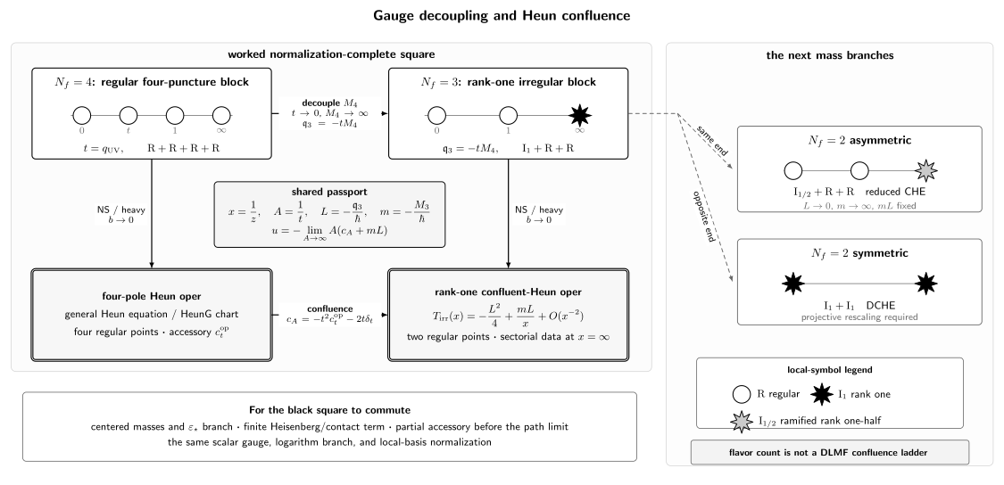
The gauge-theory decoupling ladder is labeled by the beta-function dimension $[\mathfrak q_n]=4-n$. The associated CFT or oper must additionally record which ends are regular $R$, unramified rank-one irregular $I_1$, or ramified $L_1$-only irregular $I_{1/2}$. The two standard $N_f=2$ realizations already branch: $I_1+I_1$ leads to a doubly confluent Heun problem, whereas $R+R+I_{1/2}$ is a ramified confluent problem. A named DLMF class can be assigned only after the singularity, coordinate-cover, and scalar-gauge passports are fixed.

A useful representative ledger is:

Gauge theory	Puncture or oper fingerprint	Representative quadratic differential data	Generic named scalar class
$N_f=4$	Four regular ends	Four double poles	General Heun after the probe and NS limit
$N_f=3$	$R+R+I_1$	Two regular poles and one unramified pole of degree four	Confluent Heun
$N_f=2$, realization A (symmetric)	$I_1+I_1$	Unramified degree-four poles at both ends	Doubly confluent Heun
$N_f=2$, realization B (asymmetric)	$R+R+I_{1/2}$	Two regular poles and a ramified degree-three end	Reduced CHE in Bonelli et al.; not generic DLMF CHE
$N_f=1$	$I_1+I_{1/2}$	One unramified and one ramified irregular end	Reduced DCHE in Bonelli et al.; not a generic DLMF class
$N_f=0$	$I_{1/2}+I_{1/2}$	Two $L_1$-only ramified ends	Doubly reduced DCHE; modified Mathieu after a logarithmic cover and gauge

Here $I_1$ means that $L_1$ and $L_2$ have prescribed nonzero eigenvalues, while $I_{1/2}$ means that only $L_1$ does. The half-rank notation is convenient but not universal. The mode fingerprint is the definition. Likewise, “reduced CHE,” “reduced DCHE,” and “doubly reduced DCHE” are useful labels in the cited CFT source, not additional DLMF-standard function names. The logarithmic-cover map for the pure-theory endpoint is worked out in the quantum Seiberg–Witten curve chapter.

The same-end $N_f=3\to2$ limit makes the ramified boundary concrete. Remove the remaining printed fundamental while holding

$$\mathfrak q_2 := -\lim \mathfrak q_3\mu_3 = -\lim \mathfrak q_3M_3$$

fixed. At finite $\mathfrak q_3$, choose the centered path $M_3=-\mathfrak q_2/\mathfrak q_3$. In the NS variables this sends $L\to0$ and $m\to\infty$ with

$$mL = -\frac{\mathfrak q_2}{\hbar^2}$$

fixed. The $-L^2/4$ term of $T_{\mathrm{irr}}$ disappears but the $mL/x$ term remains. On the Virasoro side $L_2$ vanishes while $L_1$ stays finite: this is the $I_{1/2}$, or $L_1$-only, boundary. If one introduces a half-rank scale by

$$\Lambda_{1/2}^2 = -4mL = \frac{4\mathfrak q_2}{\hbar^2},$$

a square-root branch has been chosen and must accompany the local solutions.

Decoupling a flavor at the opposite regular end instead creates a second unramified rank-one end and leads to realization A. A projective rescaling is then needed to display both irregular scales; under $x\mapsto\rho x$, one scale can be normalized and only their appropriate product is invariant. The words “remove the fourth and then the third flavor” are therefore insufficient: one must also say at which puncture each flavor lived.

The two $N_f=2$ rows are not a contradiction. The same four-dimensional theory has two distinct six-dimensional realizations. In a standard source convention their quadratic differentials may be represented as

$$\begin{aligned} \phi_{2,A}(z) ={}& -\frac{\Lambda^2}{z^4} -\frac{2\Lambda m_1}{z^3} +\frac{2u}{z^2} -\frac{2\Lambda m_2}{z} -\Lambda^2, \\ \phi_{2,B}(z) ={}& -\frac{m_+^2}{z^2} -\frac{m_-^2}{(z-1)^2} +\frac{2\widetilde u}{z(z-1)} +\frac{\Lambda^2}{z}. \end{aligned}$$

Realization A uses rank-one irregular states at both ends and carries a finite Abelian factor in the original normalization. Realization B uses two regular punctures and an $L_1$-only irregular end and was normalized without that factor. The instanton coordinates also differ by a finite scale convention. Equality of the underlying four-dimensional theory does not identify the two chiral blocks term by term without an explicit transform.

This branch is enough to disprove the tempting linear identification

$$N_f=4,3,2,1,0 \quad\stackrel{\text{not automatic}}{=} \quad \mathrm{GHE},\mathrm{CHE},\mathrm{DCHE},\mathrm{BHE},\mathrm{THE}.$$

The right-hand sequence is organized by scalar singularity confluence; the left-hand sequence is organized by four-dimensional beta functions. A relation between individual entries may exist after a coordinate cover, parameter specialization, and gauge transformation, but it must be demonstrated rather than inferred from the position in the list.

A moving Frobenius basis does not have an automatic limit

Coefficient convergence on compact sets away from the collision implies convergence of solutions normalized at a fixed ordinary base point. It does not imply that a Frobenius basis normalized at the moving point $x=A$ converges as printed. That point becomes irregular, so its correct local objects change:

Before collision at $x=A$	After collision at infinity
Two Frobenius powers	Two formal exponential-power branches
Small-loop monodromy	Formal monodromy combined with Stokes factors
Disk with a chosen logarithm	Overlapping Stokes sectors with a chosen direction
Frobenius-normalized connection column	Singularly renormalized, sectorial connection column

Thus a HeunG germ attached to the moving singularity does not become a confluent-Heun irregular-end germ merely by taking $A\to\infty$ in its parameters. A valid limit must specify the sign of the formal exponential, the power branch, $\arg L$, the Stokes sector, and any singular basis renormalization. The distinction between regular first-kind blocks, sectorial second-kind blocks, and Stokes matrices is developed on the irregular connection page.

A reversible decoupling passport

The $N_f=4\to3$ result can be translated safely in either direction if the following data accompany it.

Key	Four-flavor input	Three-flavor or CHE output
A · Matter	$\mu_{1,2}$ antifundamental; $\mu_{3,4}$ fundamental	Remove printed fundamental $\mu_4$
B · Scale	$t=q_{\mathrm{UV}}$	$\mathfrak q_3=-\lim t\mu_4$
C · Centering	$M_i=\mu_i-\epsilon_\Sigma/2$	$M_4=-\mathfrak q_3/t$; hold $M_3$ fixed
D · CFT state	Two regular primaries at $t,0$	$L_1=M_3\mathfrak q_3/(\epsilon_1\epsilon_2)$; $L_2=-\mathfrak q_3^2/(4\epsilon_1\epsilon_2)$
E · Chiral block	$(1-t)^{\kappa_{\mathcal H}}\widehat{\mathcal V}_{0t}$	$e^{-\alpha_1\mathfrak q_3/\varepsilon_\star}\widehat{\mathcal B}_3$
F · Probe	No probe in the bulk block	CFT: add a degenerate primary; gauge theory: choose a defect realization
G · NS exponents	$\theta_t,\theta_0$	$\theta_A=AL-m$; $\theta_\infty=-AL-m$
H · Accessory	$c_t^{\mathrm{op}}=\partial_t f$ at fixed external weights	$u=-\lim A(c_A+mL)$
I · Local endpoint	Frobenius exponents	Formal exponentials, formal monodromy, and Stokes matrices

The key letters carry the conditions and sources without widening the table:

A — matter orientation. Reflecting a flavor changes the printed mass map and the decoupling sign; see AGT §3.2 and Appendix B.

B — scale scheme. The relation $\mathfrak q_3=c_3\Lambda_3$ contains a finite convention and branch; see Gaiotto §6.

C — equivariant centering. Printed and centered finite-$t$ paths differ by $O(t\epsilon_\Sigma)$; see AGT Appendix B.2.

D — irregular state. The mode equations assume a generic Verma module and a unit-leading highest-vector coefficient; see Bonelli et al. §§2.2 and 3.2.

E — chiral equality. This is a formal-series statement at generic parameters; analytic continuation is extra. The levelwise limit is developed by Marshakov–Mironov–Morozov.

F — probe status. The null equation of the degenerate CFT insertion is exact after normalization and is generally a finite-$b$ PDE; see Bonelli et al. §3.2. Identifying that insertion with a gauge surface defect is the proposed, evidence-supported AGT extension of AGGTV, not a universal identity.

G — NS path. Here $A=1/t$, $L=-\mathfrak q_3/\hbar$, and $m=-M_3/\hbar$ on the centered path; compare Gaiotto–Teschner §7.4.

H — accessory scheme. The declared OPE power, Heisenberg factor, contact terms, and scalar gauge must be restored before comparing derivatives; see Bonelli et al. §3.2.

I — irregular endpoint. An irregular end has no single ordinary monodromy matrix; the scalar singularity classification is summarized in DLMF §31.12.

The first five rows are finite-Omega block data. The ODE rows require the extra probe and limiting assumptions. Keeping that evidentiary boundary visible prevents a coefficientwise AGT identity from being overstated as an automatic spectral theorem.

Interpretation and limitations

The decoupling limit is unusually powerful because it can be audited at three independent levels. Dimensional analysis fixes the power of the heavy mass. Individual fixed points fix its sign in a declared matter orientation. Virasoro moments fix the irregular type. The normal-form accessory remainder then tests the subleading centering and derivative conventions.

The derivation does not select a Stokes sector, an exact spectrum, or a self-adjoint realization. Once the point at infinity is irregular, formal monodromy and Stokes matrices replace an ordinary Frobenius monodromy matrix. Connection formulae additionally require sectorial normalizations, while spectral questions require cycles or boundary conditions. Those global data are developed elsewhere in the book.

The historical irregular-block formulas were proposed and tested to finite instanton order before later representation-theoretic and geometric developments greatly strengthened the framework. This page uses the coefficientwise fixed-point limit as the finite-Omega algebraic statement in the declared $A_1$ example. Claims about arbitrary class-$S$ irregular defects, convergent functions in all chambers, or exact defect spectra remain broader physical statements.

The next page makes the missing probe observable explicit: it separates a degenerate insertion and its BPZ equation from the several gauge-side surface-defect constructions that can realize a quantum curve.

Common pitfalls

Taking $t\to0$ at fixed mass. That is the ordinary weak-coupling cusp of the conformal theory. A finite irregular scale requires the correlated limit $t\mu_4=O(1)$ with the heavy mass diverging.

Forgetting the matter-orientation sign. A printed fundamental box is asymptotic to $-\mu$, whereas a printed antifundamental box is asymptotic to $+\mu$. The definition of the lower-flavor fugacity must follow the actual box factor.

Using printed and centered masses interchangeably at subleading order. They give the same limiting $\mathfrak q_3$ but different finite-$t$ paths. The oper collision and accessory remainder use centered masses.

Setting the Heisenberg factor to one because $t\to0$. Its exponent diverges like $1/t$, leaving a finite exponential. That exponential shifts the NS scale derivative.

Calling the bulk irregular block a confluent-Heun solution. The bulk block has no probe coordinate. A degenerate insertion, fusion choice, classical reduction, and scalar gauge are still required.

Equating flavor number with a named Heun equation. Lower-flavor theories can have inequivalent puncture realizations, including ramified ones. Classify nonzero modes and pole orders before naming the scalar equation.

Exercises

1. Dimensional scale matching

Suppose $\mathfrak q_n=c_n\Lambda_n^{4-n}$ and a heavy printed fundamental mass is decoupled. Show that $\mathfrak q_{n-1}=-\mu \mathfrak q_n$ has the correct dimension and write the corresponding relation between $\Lambda_{n-1}$ and $\Lambda_n$.

Solution

Since $[\mu]=1$ and $[\mathfrak q_n]=4-n$,

$$[-\mu \mathfrak q_n] = 5-n = 4-(n-1) = [\mathfrak q_{n-1}].$$

Thus

$$c_{n-1}\Lambda_{n-1}^{5-n} = -\mu\,c_n\Lambda_n^{4-n}.$$

The sign and ratio $c_n/c_{n-1}$ can be absorbed into a chosen root of the strong-coupling scale, but that choice must remain fixed in later comparisons.

2. A box-by-box decoupling audit

Starting from the declared fundamental factor, prove the $N_f=4\to3$ limit at a fixed diagram pair. Repeat the argument for a heavy printed antifundamental and determine the new scale sign.

Solution

For $k=|\boldsymbol Y|$,

$$\prod_{\alpha,s} [\phi(a_\alpha,s)-\mu+\epsilon_\Sigma] = (-\mu)^k[1+O(\mu^{-1})].$$

Therefore $t^kz_{\mathrm{fund}}\to(-t\mu)^k=\mathfrak q_3^k$. An antifundamental factor is $\prod_{\alpha,s}[\phi(a_\alpha,s)+\mu] =\mu^k[1+O(\mu^{-1})]$, so its finite lower-flavor coordinate is $\mathfrak q_3=+t\mu$.

3. The collision is not a regular OPE

Use $p_t=(M_3+M_4)/2$, $p_0=(M_3-M_4)/2$, and $M_4=-\mathfrak q_3/t$ to find the sum and difference of the colliding masses. Explain which quantity remains finite and which one supplies the irregular scale.

Solution

One finds

$$p_t+p_0=M_3, \qquad p_t-p_0=M_4=-\frac{\mathfrak q_3}{t}.$$

The finite sum supplies the remaining flavor parameter. The divergent difference combines with the vanishing separation $t$ to leave the finite moment $\mathfrak q_3$. Holding both $p_t$ and $p_0$ finite would remove that moment and give an ordinary OPE degeneration.

4. Irregular-mode eigenvalues

Insert $\mu_{\mathcal I}=-M_3/\varepsilon_\star$ and $\Lambda_{\mathcal I}=-\mathfrak q_3/\varepsilon_\star$ into the book’s rank-one ket constraints. Recover the dimensionful eigenvalues printed above.

Solution

The first moment is

$$\mu_{\mathcal I}\Lambda_{\mathcal I} = \frac{M_3\mathfrak q_3}{\varepsilon_\star^2} = \frac{M_3\mathfrak q_3}{\epsilon_1\epsilon_2},$$

and the second is

$$-\frac{\Lambda_{\mathcal I}^2}{4} = -\frac{\mathfrak q_3^2}{4\epsilon_1\epsilon_2}.$$

Both are dimensionless, as Virasoro eigenvalues must be.

5. The surviving Heisenberg exponential

Using $\alpha_t=(\mu_3+\mu_4)/(2\varepsilon_\star)$ and $\mathfrak q_3=-t\mu_4+o(1)$, evaluate $\lim\kappa_{\mathcal H}\Log(1-t)$.

Solution

The divergent part is

$$\kappa_{\mathcal H} = 2\alpha_1(Q_{\mathrm L}-\alpha_t) = \frac{\alpha_1\mathfrak q_3}{\varepsilon_\star t}+O(1).$$

Since $\Log(1-t)=-t+O(t^2)$,

$$\lim_{t\to0} \kappa_{\mathcal H}\Log(1-t) = -\frac{\alpha_1\mathfrak q_3}{\varepsilon_\star}.$$

Exponentiating gives the finite factor on the page.

6. The accessory remainder under inversion

Derive $c_A=-t^2c_t^{\mathrm{op}}-2t\delta_t$ directly from $x=1/z$, and then express $u=-\lim A(c_A+mL)$ in the original $t$ coordinate.

Solution

For a Möbius transformation the Schwarzian vanishes, so $T_x(x)=x^{-4}T_z(1/x)$. Near $x=A=1/t$,

$$\frac{x^{-4}\delta_t}{(x^{-1}-t)^2} = \frac{\delta_t}{(x-A)^2} -\frac{2t\delta_t}{x-A}+O(1),$$

while

$$\frac{x^{-4}c_t^{\mathrm{op}}}{x^{-1}-t} = -\frac{t^2c_t^{\mathrm{op}}}{x-A}+O(1).$$

Adding the residues gives the stated $c_A$. Since $A=1/t$,

$$u = \lim_{t\to0} \left[ t c_t^{\mathrm{op}} +2\delta_t -\frac{mL}{t} \right].$$

7. Two realizations of the same flavor number

Read the two displayed $N_f=2$ quadratic differentials at $z=0$ and $z=\infty$. Determine their pole degrees as quadratic differentials and explain why only realization A is generically doubly confluent Heun in the displayed coordinate.

Solution

In realization A, $\phi_{2,A}$ has a fourth-order pole at $z=0$. Under $w=1/z$, the constant term $-\Lambda^2$ becomes a fourth-order pole at $w=0$, so both ends are unramified rank one. This is the generic doubly confluent profile.

In realization B, $z=0$ and $z=1$ are regular singular ends. The term $\Lambda^2/z$ becomes a third-order pole of the quadratic differential at infinity, hence an $L_1$-only ramified irregular end. It does not have the two rank-one ends of generic DCHE, and it does not have the unramified rank-one end of generic CHE without an additional cover or specialization.

8. Audit the order of limits

Starting from $\Lambda_{\mathcal I}=-\mathfrak q_3/\varepsilon_\star$ and $\mu_{\mathcal I}=-M_3/\varepsilon_\star$, take the book’s NS limit and recover $(L,m)$. Then show what finite shift appears in $m$ if one incorrectly holds the printed $\mu_3$ fixed while comparing with a path that holds $M_3$ fixed.

Solution

Because $\varepsilon_\star=b\hbar$,

$$b\Lambda_{\mathcal I} = -\frac{\mathfrak q_3}{\hbar} =L, \qquad b\mu_{\mathcal I} = -\frac{M_3}{\hbar} =m.$$

But $M_3=\mu_3-\epsilon_\Sigma/2$ and $\epsilon_\Sigma\to\hbar$. Holding $\mu_3$ rather than $M_3$ fixed would give

$$m = -\frac{\mu_3}{\hbar} +\frac12$$

instead of treating $m$ as the fixed centered datum. The one-half is an equivariant centering shift. It must be translated before the two routes through the limiting square can be compared.

References

• D. Gaiotto, “Asymptotically Free $\mathcal N=2$ Theories and Irregular Conformal Blocks”, Journal of Physics: Conference Series 462 (2013) 012014. The introduction formulates asymptotically free limits as heavy-mass collisions. Sections 2–6 give the $N_f=0,1,2,3$ quadratic differentials, Virasoro-mode constraints, instanton-scale conventions, and the two inequivalent $N_f=2$ realizations. The paper presents the irregular-block identifications as proposals checked to finite level in its examples.
• L. F. Alday, D. Gaiotto, and Y. Tachikawa, “Liouville Correlation Functions from Four-dimensional Gauge Theories”, Letters in Mathematical Physics 91 (2010), 167–197. Section 3.2 and Appendix B fix the regular four-flavor mass orientation, equivariant shifts, box convention, and Heisenberg factor whose limit is taken here.
• L. F. Alday, D. Gaiotto, S. Gukov, Y. Tachikawa, and H. Verlinde, “Loop and Surface Operators in $\mathcal N=2$ Gauge Theory and Liouville Modular Geometry”, Journal of High Energy Physics 01 (2010) 113. Section 2 proposes the degenerate-insertion/surface-defect bridge used only as a status marker here; the next page distinguishes concrete defect realizations.
• A. Marshakov, A. Mironov, and A. Morozov, “On Non-conformal Limit of the AGT Relations”, Physics Letters B 682 (2009), 125–129. Equations (8)–(30) construct lower-flavor irregular vectors as levelwise limits of regular Virasoro blocks and distinguish the physical threshold scale from a convention-dependent distribution of powers between bra and ket. The inverse-Shapovalov formulas assume a generic Verma module.
• D. Gaiotto and J. Teschner, “Irregular Singularities in Liouville Theory and Argyres–Douglas Type Gauge Theories, I”, Journal of High Energy Physics 12 (2012) 050. Sections 2–3 systematize collision limits, irregular vectors, and their relation to wild Hitchin data.
• G. Bonelli, C. Iossa, D. Panea Lichtig, and A. Tanzini, “Irregular Liouville Correlators and Connection Formulae for Heun Functions”, Communications in Mathematical Physics 397 (2023), 635–727. The paper develops irregular Liouville correlators and relates their semiclassical degenerate limits to confluent Heun connection problems, with normalization and sector data kept explicit.
• NIST Digital Library of Mathematical Functions, §31.12, “Confluent Forms of Heun’s Equation”. This is the reference classification for confluent, doubly confluent, biconfluent, and triconfluent scalar Heun equations. It classifies differential-equation singularities, not gauge-theory beta functions.