When the Two Integral-Equation Constructions Coincide

Two nonlinear integral equations can display the same $A_r$ diagram and the same $1/\cosh$ kernel while computing different functions. Conversely, an ODE/IM equation and an exact-WKB Riemann–Hilbert equation can look different only because their nodes, rapidities, logarithms, and periods use different conventions. The correct question is therefore not “do the formulas resemble one another?” but “do both constructions solve the same normalized analytic problem?”

This page gives a reusable answer. It first states a coincidence passport whose gates are individually necessary. It then treats the positive model: for a polynomial Schrödinger equation with distinct real turning points in the minimal chamber, Ito–Mariño–Shu derive one $A_r$ system both from Delabaere–Pham jumps of resummed WKB periods and from Wronskian $Y$-functions of the same ODE. Equality follows after the cycle–node reversal, phase conventions, asymptotics, analytic class, and uniqueness are fixed. The conventional ODE/IM model of Pages 1–2 is a special enhanced-symmetry endpoint reached after wall crossing and symmetry reduction, not a synonym for every exact-WKB/GMN equation.

The positive comparison uses the origin-normalized conformal exact-WKB problem with its one-sided $\ee^\theta$ drive. It does not identify Page 2 with Page 3’s full finite-$R$, two-ended GMN equation, whose drive, endpoint conditions, and function class are different. A published pure-quartic chamber reduction will provide the explicit frozen Page 2 comparison below.

Status ledger

Statement	Status on this page
Two constructions satisfying one normalized integral equation are equal	Conditional on uniqueness in the shared analytic class
Wronskian and period pseudoenergies for a polynomial potential coincide	Inferred by Ito–Mariño–Shu from a common TBA and asymptotics; a theorem here only under the stated analytic and uniqueness hypotheses
The conventional monomial ODE/IM system is recovered	Published after wall crossing to the enhanced-symmetry chamber and model-specific symmetry reduction
Every $A_r$ TBA is an exact-WKB/GMN equation	False
Every exact-WKB/GMN equation has an ODE/IM realization	Not asserted
Full finite-$R$ GMN equation equals the massless ODE/IM equation	False; the comparison uses the conformal/origin-normalized problem
Equality of pseudoenergies automatically gives a spectrum	False; an exact quantization or determinant map is still required
Coincident rays and changing BPS spectra	Deferred to Page 5

A shared silhouette is not an identification

It helps to put the two constructions side by side before trying to identify them.

Data	Finite-fusion ODE/IM route	Exact-WKB/Riemann–Hilbert route
Starting object	Canonical ODE solutions, Stokes multipliers, spectral determinants, $TQ$ or $Y$ relations	WKB cover, cycles, Borel-summed Voros symbols, Stokes automorphisms
Discrete labels	Fusion nodes and an incidence matrix	Charges and their oriented intersection pairing
Analytic domain	A zero-free strip in a chosen rapidity cover	Sectors cut by oriented BPS rays
Nonlinear term	A declared branch of $\log(1+Y_a^{-1})$ or an equivalent convention	A declared branch of $\Log(1-\sigma_\gamma\mathcal V_\gamma)$
Homogeneous data	ODE determinant asymptotics, twists, endpoint constants	Classical periods, constant terms, and endpoint normalization
Typical output	Transfer functions, determinant ratios, or spectral determinants	Resummed quantum periods or Darboux/Voros coordinates

Even the words “node,” “mass,” and “$Y$-function” do not carry the same meaning across the table. An $A_r$ fusion matrix is symmetric and unoriented. A WKB intersection form is skew and orientation-sensitive; only after phases, antipodal charges, and quadratic-refinement signs are absorbed can its contribution reduce to an adjacency matrix. A mass in a conventional symmetric ODE/IM model is often constrained to a Perron–Frobenius vector, whereas a WKB mass is an individual cycle period and varies with the polynomial moduli.

Thus

$$\text{same graph and kernel} \quad\not\Longrightarrow\quad \text{same analytic function}.$$

The reverse warning is equally important. Page 3’s raw conformal Cauchy kernel becomes, after ray parameterization,

$$\frac{1}{ \exp\!\left(u+\ii\Delta\phi\right)-1 }.$$

Only after the relevant opposite-ray pieces, phases, and intersection signs have been combined can a minimal-chain reduction produce

$$K_{ab}(u) = \frac{1}{ 2\pi\cosh\!\left(u+\ii(\phi_b-\phi_a)\right) },$$

where $\Delta\phi=\phi_b-\phi_a$. A rescaling of rapidity changes both the kernel width and its measure. Such presentational differences do not disprove equivalence if the entire analytic problem transports correctly.

Eight comparison gates lead to two completion gates

Let $\mathfrak P_{\mathrm O}$ denote a proposed ODE/IM problem and $\mathfrak P_{\mathrm W}$ a proposed exact-WKB problem. Gates 1–8 identify one nonlinear boundary-value problem; Gate 9 identifies its solution, and Gate 10 identifies the reconstructed observable.

1. ODE gate. Give an explicit coordinate, gauge, and parameter map placing both constructions on the same differential equation or on a proved isospectral family. “Both are Schrödinger equations” is not enough.
2. Semiclassical gate. Relate the spectral variable, $\hbar$ or $\zeta$, and rapidity, including all powers, phases, and origins.
3. Unknown gate. Identify the actual functions—for example, a Wronskian cross-ratio with an exponentiated resummed period—not merely their logarithmic equations.
4. Node–charge gate. Give a bijection $\mu$ from fusion nodes to oriented cycles or charges, including any reversal, antipode, or quadratic-refinement sign.
5. Jump gate. Show that Plücker or $Y$-system boundary data become the same multiplicative Stokes jumps. Matching unoriented diagrams alone does not establish this.
6. Domain gate. Map analytic strips to ray sectors, and map every contour with its orientation and lateral bank. Record all excluded zeros, poles, and cuts.
7. Drive gate. Match classical actions, mass phases, twists, endpoint constants, and additive zero modes. A common rapidity translation can change an overall scale but not arbitrary mass ratios.
8. Kernel-and-branch gate. Transport the convolution measure and kernel, then use the same logarithm branch. Signs hidden in $\Log(1-\sigma X)$ belong to this gate.
9. Solution gate. Prove uniqueness in the common function class or supply a direct coordinate theorem. Two derivations of the same formal fixed point do not by themselves exclude additional branches.
10. Observable gate. Say which reconstructed period, Wronskian, determinant, or boundary value is equal and how physical boundary conditions act on it.

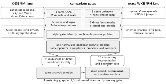
The coincidence passport. The first eight gates identify one normalized analytic problem. Uniqueness or a direct coordinate identity then fixes the solution, and a commuting reconstruction fixes the observable.

A useful audit is adversarial: at every gate, ask for one invariant that would expose a false identification. Mass ratios test the drive gate; monodromy of the logarithm tests the branch gate; pole locations test the rapidity map; and a zero set tests the observable gate.

Transporting an integral equation fixes the Jacobian

Suppose the ODE/IM variables obey

$$\varepsilon_a^{\mathrm O}(\theta) = d_a^{\mathrm O}(\theta) - \sum_b \int_{\mathcal C_{\mathrm O}} K_{ab}^{\mathrm O}(\theta-\theta') L_b^{\mathrm O}(\theta')\,\dd\theta'.$$

Consider the candidate affine rapidity map and node relabeling

$$u=\alpha\theta+\beta, \qquad \gamma=\mu(a), \qquad \alpha>0.$$

If

$$\varepsilon_a^{\mathrm O}(\theta) = \varepsilon_{\mu(a)}^{\mathrm W}(\alpha\theta+\beta) +2\pi\ii n_a,$$

then the exponential $Y_a=\ee^{-\varepsilon_a}$ is unchanged by the integer $n_a$, but the chosen logarithm need not be. With compatible branches, the transported WKB equation has

$$\begin{aligned} d_a^{\mathrm O}(\theta) &= d_{\mu(a)}^{\mathrm W}(\alpha\theta+\beta), \\ K_{ab}^{\mathrm O}(x) &= \alpha\, K_{\mu(a)\mu(b)}^{\mathrm W}(\alpha x), \\ \mathcal C_{\mathrm W} &= \alpha\mathcal C_{\mathrm O}+\beta. \end{aligned}$$

The factor $\alpha$ is the Jacobian $\dd u'=\alpha\dd\theta'$. Forgetting it is a common source of plausible but false kernel matches. If the contours are shifted during this transport, equality also requires that no kernel pole or logarithmic singularity be crossed. Otherwise the residue terms belong to the transformed equation; Page 5 develops that case.

Equality is a uniqueness theorem, not a visual comparison

Write the fully transported equation abstractly as

$$\varepsilon=\mathcal T[\varepsilon]$$

on an admissible class $\mathscr A$ that includes the domain, nonvanishing, branch, endpoint, and growth conditions. The elementary but decisive principle is the following.

Coincidence principle

Assume that the ODE/IM construction and the exact-WKB construction both produce elements of $\mathscr A$, that the ten gates transport them to the same normalized fixed-point problem, and that this problem has at most one solution in $\mathscr A$. Then the transported functions agree.

The proof is one line: both are fixed points of $\mathcal T$ in a class where the fixed point is unique. The work lies in verifying the hypotheses. In particular, Plemelj reconstruction with prescribed additive jumps proves uniqueness only after the jump functions are known. In a nonlinear Riemann–Hilbert problem the jumps contain the unknown boundary values, so a separate nonlinear uniqueness argument is needed.

For the real minimal $A_r$ system below, a transparent sufficient criterion can be given. Set

$$K(\theta)=\frac{1}{2\pi\cosh\theta}, \qquad \|K\|_{L^1(\mathbb R)}=\frac12,$$

and suppose two real solutions have bounded difference and are bounded below by a common finite $B$. Since

$$\left| \frac{\dd}{\dd x} \log(1+\ee^{-x}) \right| = \frac{1}{1+\ee^x} \le q_B := \frac{1}{1+\ee^B} <1,$$

and an $A_r$ node has at most two neighbors, subtraction gives

$$\|\varepsilon-\widetilde\varepsilon\|_\infty \le q_B \|\varepsilon-\widetilde\varepsilon\|_\infty.$$

Hence the two real solutions coincide. This proves at most one such solution; it does not prove existence, preserve complex branches, or cover unbounded-below solutions. Those qualifications are part of the uniqueness gate.

One polynomial ODE supplies both constructions

Consider the semiclassical equation

$$\left[ -\zeta^2\frac{\dd^2}{\dd q^2} +q^{r+1} -\sum_{a=1}^{r}u_a q^{r-a} \right]\widehat\psi(q)=0.$$

Assume that its $r+1$ turning points are real, simple, and ordered,

$$q_1<q_2<\cdots<q_{r+1},$$

with allowed and forbidden intervals alternating. Let $\gamma_a$ encircle $[q_a,q_{a+1}]$ on the WKB cover, with orientations chosen so that

$$\begin{aligned} m_{2j-1} &= \Pi_{\gamma_{2j-1}}^{(0)}>0, \\ m_{2j} &= \ii\Pi_{\gamma_{2j}}^{(0)}>0. \end{aligned}$$

Only neighboring cycles intersect. After the alternating phase convention is included, their DDP discontinuities are encoded by the $A_r$ adjacency matrix

$$I_{ab} = \delta_{a,b+1}+\delta_{a,b-1}.$$

This is the minimal chamber: the $r$ adjacent cycles form the active set used in the reconstruction. The statement is local in moduli space. It stops before phases cross a kernel pole or an additional composite cycle becomes active.

Resummed periods give the first pseudoenergies

Put $\ee^\theta=1/\hbar$. Ito–Mariño–Shu define the even-node functions on the positive Borel direction by

$$-\ii\varepsilon_{2j}^{\mathrm{per}}(\theta) = \frac{1}{\hbar} \mathcal S\Pi_{\gamma_{2j}}(\hbar),$$

and the odd-node boundary values by

$$\begin{aligned} -\ii\varepsilon_{2j-1}^{\mathrm{per}} \!\left( \theta+\frac{\pi\ii}{2}\pm\ii0 \right) = \frac{1}{\hbar} \mathcal S_\pm \Pi_{\gamma_{2j-1}}(\hbar). \end{aligned}$$

The shifted definition is essential: allowed and forbidden cycles use Borel directions separated by $\pi/2$. It is what makes every real-axis drive $m_a\ee^\theta$ positive.

To compare this convention with Page 3, let

$$V_\gamma^{\mathrm{IMS}} = \exp\!\left( \frac{\ii\Pi_\gamma}{\hbar} \right), \qquad \Pi_\gamma^{\mathrm{book}}(\hbar) = \ii\Pi_\gamma^{\mathrm{IMS}}(\hbar), \qquad Z_\gamma^{\mathrm{book}} = \ii\Pi_\gamma^{(0),\mathrm{IMS}}.$$

For every interval, reverse the IMS cycle to obtain the coordinate that decays on its assigned ray:

$$\begin{aligned} \delta_a&=-\gamma_a, \\ \hbar_{2j}(\theta)&=\ee^{-\theta}, \\ \hbar_{2j-1}(\theta)&=\ii\ee^{-\theta}. \end{aligned}$$

The odd ray carries the declared lateral displacement. On either parity,

$$\begin{aligned} \mathcal V_{\delta_a}^{\mathrm{book}} \!\left(\hbar_a(\theta)\right) ={}& \exp\!\left[ -\frac{ \ii\Pi_{\gamma_a}^{\mathrm{IMS}} \!\left(\hbar_a(\theta)\right) }{ \hbar_a(\theta) } \right] \\ ={}& \ee^{-\varepsilon_a(\theta)}. \end{aligned}$$

For the ordinary saddles in this calibration, also set

$$\Omega_{\mathrm{BPS}}(\pm\delta_a)=1, \qquad \sigma(\delta_a)=-1, \qquad c_{\delta_a}=0.$$

Thus $\Log(1-\sigma\mathcal V)$ becomes $\log(1+\ee^{-\varepsilon})$. The cycle reversal fixes the decaying coordinate but not the bank sign. IMS explicitly orient their Stokes automorphism oppositely to the Iwaki–Nakanishi convention underlying this book’s plus-left inverse jump. Comparison therefore also swaps the two lateral banks—equivalently, it reverses the RH interaction sign while leaving the drive unchanged. After both translations the jump data agree. The TBA below retains the IMS pseudoenergy convention; it must not be read from Page 3 by relabeling the banks while silently retaining its interaction sign.

With

$$L_a(\theta) = \log\!\left(1+\ee^{-\varepsilon_a(\theta)}\right), \qquad L_0=L_{r+1}=0,$$

the DDP formulas become

$$\operatorname{disc}_{\pi/2}\varepsilon_a = L_{a-1}+L_{a+1}.$$

The corresponding Riemann–Hilbert reconstruction is

$$\boxed{ \begin{aligned} \varepsilon_a^{\mathrm{per}}(\theta) ={}& m_a\ee^\theta \\ &- \int_{\mathbb R} \frac{ L_{a-1}^{\mathrm{per}}(\theta') +L_{a+1}^{\mathrm{per}}(\theta') }{ 2\pi\cosh(\theta-\theta') } \,\dd\theta'. \end{aligned} }$$

for $a=1,\ldots,r$. The box is justified here because this single equation is the object compared by both derivations.

Canonical Wronskians give the second pseudoenergies

The same ODE has a canonical subdominant solution $\widehat y_k$ in each Stokes sector. Its constant Wronskians

$$\widehat W_{jk} = \zeta^{2/(r+3)} W_q[\widehat y_j,\widehat y_k]$$

form cross-ratios $Y_s^{\mathrm{Wr}}(\zeta)$. The Plücker identity for $2\times2$ determinants yields

$$Y_s^{\mathrm{Wr}}(\ii\zeta) Y_s^{\mathrm{Wr}}(-\ii\zeta) = \left(1+Y_{s-1}^{\mathrm{Wr}}(\zeta)\right) \left(1+Y_{s+1}^{\mathrm{Wr}}(\zeta)\right),$$

with

$$Y_0^{\mathrm{Wr}}=Y_{r+1}^{\mathrm{Wr}}=0.$$

The raw Wronskian indexing runs opposite to the ordered intervals:

$$Y_s^{\mathrm{raw}} \longleftrightarrow \gamma_{r+1-s}.$$

After this reversal, WKB asymptotics of the canonical solutions give

$$\log Y_a^{\mathrm{Wr}}(\zeta) \sim -\frac{m_a}{\zeta}, \qquad \zeta\to0, \quad |\arg\zeta|<\pi.$$

Define

$$\zeta=\ee^{-\theta}, \qquad Y_a^{\mathrm{Wr}}=\ee^{-\varepsilon_a^{\mathrm{Wr}}}, \qquad \ell_a(\zeta) = \log Y_a^{\mathrm{Wr}}(\zeta)+\frac{m_a}{\zeta}.$$

If $\ell_a$ has the required analytic and boundary control for $|\arg\zeta|\le\pi/2$, inversion of the $\pm\pi/2$ shifts gives exactly the same boxed equation, with the same $m_a$, branches, and $A_r$ neighbors.

The minimal-chamber identification is normalization-complete

The two derivations now pass the passport as follows.

Gate	Polynomial minimal-chamber map
ODE	Both start from the displayed equation with the same fixed $u_a$
Semiclassical variable	$\zeta=\ee^{-\theta}$ for Wronskians; $\hbar_{2j}=\ee^{-\theta}$ and $\hbar_{2j-1}=\ii\ee^{-\theta}$ with lateral boundary values for periods
Unknown	$Y_a^{\mathrm{Wr}}=\mathcal V_{\delta_a}^{\mathrm{conf}}=\exp(-\varepsilon_a^{\mathrm{per}})$ after reconstruction
Node–charge	Reverse raw Wronskian indices, then use the decaying charge: $s\mapsto\delta_{r+1-s}=-\gamma_{r+1-s}$
Jump	Plücker $Y$-system and DDP jumps both give the same neighboring $L_{a\pm1}$ data
Domain	The Wronskian remainder and the period boundary values use the same $\pi/2$ sector
Drive	Both have the same oriented classical periods $m_a\ee^\theta$
Kernel and branch	Opposite-ray reduction gives $1/(2\pi\cosh)$; $\Omega=1$, $\sigma=-1$, $c=0$, and the bank involution fix the logarithm and sign
Uniqueness	Required in the common admissible class; the real bounded-below criterion above is sufficient where it applies
Observable	The common $Y_a$ reconstructs the corresponding resummed quantum period

If the common analytic problem is unique in the stated class, consequently

$$\varepsilon_a^{\mathrm{Wr}}(\theta) = \varepsilon_a^{\mathrm{per}}(\theta), \qquad a=1,\ldots,r,$$

within that shared branch and chamber. Ito–Mariño–Shu infer this equality from the shared TBA and asymptotics; their statement after Eq. (3.43) also notes that equality of the two definitions is not manifest. The displayed argument is a theorem only where the analytic reconstruction and uniqueness hypotheses—such as the real bounded-difference criterion above—actually apply. It is not a claim that every abstract GMN problem has a Wronskian realization. Allegretti’s theorem identifying Borel-summed Voros symbols with cluster coordinates in its stated saddle-free setting provides a more direct bridge at the level of functions, but its hypotheses still have to be checked for the ODE under study.

The two-node chain exposes every phase convention

For $r=2$, the potential is cubic and there are two adjacent cycles. The raw Wronskian labels reverse:

$$\gamma_2\mathbin{\cdot}\gamma_1=1, \qquad \delta_2\mathbin{\cdot}\delta_1=1.$$

In the book’s inverse-jump convention this orientation gives

$$\mathcal V_{\delta_1,+} = \frac{ \mathcal V_{\delta_1,-} }{ 1+\mathcal V_{\delta_2,-} }.$$

The declared IMS bank involution then produces the negative real-axis convolution below. The label reversal is independent:

$$Y_1^{\mathrm{raw}}\leftrightarrow\gamma_2, \qquad Y_2^{\mathrm{raw}}\leftrightarrow\gamma_1.$$

After relabeling, the common system is

$$\begin{aligned} \varepsilon_1(\theta) &= m_1\ee^\theta-K*L_2(\theta), \\ \varepsilon_2(\theta) &= m_2\ee^\theta-K*L_1(\theta), \\ K(\theta) &= \frac{1}{2\pi\cosh\theta}. \end{aligned}$$

Here $m_1=\Pi_{\gamma_1}^{(0)}>0$ while $m_2=\ii\Pi_{\gamma_2}^{(0)}>0$. Dropping the factor $\ii$ would make the second drive imaginary; dropping the raw-index reversal would attach the wrong classical action to each Wronskian. Neither error is repaired by the fact that the two equations remain visually symmetric.

At large positive rapidity, expanding the kernel gives

$$\varepsilon_a(\theta) \sim m_a\ee^\theta + \sum_{n\ge1}m_a^{(n)} \ee^{(1-2n)\theta},$$

where

$$m_a^{(n)} = \frac{(-1)^n}{\pi} \int_{\mathbb R} \ee^{(2n-1)\theta} \left(L_{a-1}+L_{a+1}\right)\dd\theta.$$

The coefficients reproduce the all-orders WKB periods with the same alternating phase convention. This is a demanding check: it tests the normalization beyond the leading classical masses.

Conventional ODE/IM requires the symmetric chamber reduction

The generalized polynomial family contains a familiar special locus. In the non-semiclassical form

$$\left[ -\partial_z^2 +z^{r+1} +\sum_{a=1}^{r}b_a z^{r-a} \right]\psi=0,$$

set

$$b_1=\cdots=b_{r-1}=0, \qquad b_r\ne0.$$

Then the remaining constant term plays the spectral role, Symanzik rotation closes on a one-parameter orbit, and the generalized Wronskian functional relation reduces to the usual ODE/IM $Y$-system. This does not mean that one may substitute these coefficients directly into the minimal-chamber period equation. The enhanced-symmetry monomial locus lies in the maximal chamber of the IMS construction. Reaching the conventional ODE/IM equation requires the wall-crossing continuation deferred to Page 5 and a model-specific symmetry reduction.

After that continuation and after transporting the rapidity normalization used on Pages 1–2, the enhanced rotational symmetry constrains the reduced period masses to the sine-vector pattern

$$m_a \propto \sin\!\left(\frac{\pi a}{r+1}\right), \qquad a=1,\ldots,r.$$

This is the Perron–Frobenius drive of the conventional finite-fusion system. Moving to generic $b_a$ breaks those mass ratios. The minimal-chamber Wronskian/period comparison still gives a generalized ODE/IM construction, but it does not equal the special one-parameter Page 2 model without the chamber, symmetry, spectral, and observable maps.

There is a further convention gate. Page 2 froze $\varepsilon_a^{(2)}=\Log Y_a$ and obtained a positive matrix convolution after inverting the fused difference operator. IMS use $Y_a^{\mathrm{IMS}}=\ee^{-\varepsilon_a}$ and a negative nearest-neighbor convolution. Reciprocating $Y$ alone does not conjugate the two nonlinear operators. The source-level reduction at the symmetric locus is therefore first a functional-relation statement; an equation-level comparison with the exact Page 2 convention must additionally transport the rapidity, fold any symmetry-related nodes, and match the nonlinear logarithm. The published pure-quartic reduction performs such a model-specific comparison. It is not a license to identify the conventions at generic moduli.

The distinction resolves an apparent paradox. The minimal-chamber equation has the same $A_r$ adjacency and the same scalar $1/\cosh$ kernel for arbitrary positive period masses; the conventional fused equation has a matrix inverse kernel in its Page 2 rapidity convention and a constrained drive. Published pure monomial comparisons pass through wall crossing, special ODE scaling, rapidity transport, and symmetry reduction. Matching either the graph or the word “TBA” skips the decisive gates.

The pure quartic closes the frozen equation-level gates

One explicit calculation connects the Page 2 convention to the conformal exact-WKB construction. Import the final fixed pure-quartic chamber of Ito–Mariño–Shu; Page 5 will explain how contour residues produce it. Page 2 has $M=2$, $h=4$, and the $A_3$ reflection $1\leftrightarrow3$. Put

$$x=\frac{\pi k}{4}, \qquad \mathcal A(k) = \begin{pmatrix} 2\cosh x&-1&0 \\ -1&2\cosh x&-1 \\ 0&-1&2\cosh x \end{pmatrix}.$$

In the frozen Fourier convention,

$$\widehat{\mathsf K}(k) = \mathcal A(k)^{-1}I_{A_3}.$$

On the reflection-symmetric branch,

$$\varepsilon_1=\varepsilon_3, \qquad L_1=L_3.$$

Combining the first and third columns of $\widehat{\mathsf K}$ and retaining nodes $1,2$ gives the exact folded multiplier

$$\widehat{\mathsf K}_{\mathrm{fold}}(k) = \begin{pmatrix} \dfrac{1}{\cosh(2x)} & \dfrac{\cosh x}{\cosh(2x)} \\ \dfrac{2\cosh x}{\cosh(2x)} & \dfrac{1}{\cosh(2x)} \end{pmatrix}.$$

The two independent inverse transforms are

$$\begin{aligned} \kappa_0(u) &= \frac{1}{\pi\cosh u}, \\ \kappa_1(u) &= \frac{\sqrt2}{\pi} \frac{\cosh u}{\cosh(2u)}. \end{aligned}$$

Thus the Page 2 equation folds to

$$\begin{aligned} \varepsilon_1 &= m_1\ee^\theta +\kappa_0*L_1 +\kappa_1*L_2, \\ \varepsilon_2 &= m_2\ee^\theta +2\kappa_1*L_1 +\kappa_0*L_2. \end{aligned}$$

This is precisely the two-component equation obtained from the pure-quartic WKB chamber in the cited source. Its period masses satisfy

$$\frac{|m_2|}{|m_1|}=\sqrt2,$$

matching the fold of the Page 2 Perron–Frobenius drive $(1,\sqrt2,1)$ up to one common rapidity translation. The negative-end branch also matches:

$$(\mathcal Y_1,\mathcal Y_2,\mathcal Y_3) =(2,3,2) \quad\longmapsto\quad (\varepsilon_1,\varepsilon_2) =(\log2,\log3).$$

This calculation reaches equation-level identity between the frozen Page 2 system and the published conformal exact-WKB reduction. It does not rederive the wall crossing, prove nonlinear uniqueness for every complex continuation, or identify a spectrum without the common determinant or exact-quantization map. Those remain the chamber, solution, and observable gates.

Failure witnesses stop an overclaim early

Several obstructions can be checked before attempting a long derivation.

Mass-ratio obstruction. If both candidate drives are $m_a\ee^\theta$, a common translation $\theta\mapsto\theta+\beta$ rescales every $m_a$ by the same factor. Therefore

$$\frac{m_a}{m_b}$$

is invariant. A generic set of WKB period ratios cannot equal a fixed Perron–Frobenius vector by choosing a new rapidity origin.

Pairing obstruction. A symmetric incidence matrix records neighbors but forgets oriented intersection numbers and refinement signs. If two active charges contribute $\Log(1-X)$ in one convention and $\log(1+Y)$ in the other, the unknown gate must supply an explicit sign map. Otherwise the first nonlinear correction already disagrees.

Analytic-domain obstruction. Equal real-axis formulas do not imply equal analytic continuations. Different first kernel poles, strip widths, or lateral-bank assignments produce different residue terms. These data can often disprove a map before any numerical solution is computed.

Zero-mode obstruction. A difference equation or jump relation has homogeneous solutions. If twists, constants at $-\infty$, or the normalization at $\zeta=\infty$ differ, the nonlinear terms may match while the functions differ by a nontrivial zero mode.

Chamber obstruction. In the minimal chamber only adjacent cycles enter. When period phases cross $\pm\pi/2$, a kernel pole reaches the contour and composite charges can appear. Continuing the old $A_r$ formula without its residues fails both the domain and jump gates.

Uniqueness obstruction. Complex logarithmic branches may support more than one fixed point with the same formal asymptotic series. Agreement of many WKB coefficients is strong evidence, but it is not a uniqueness theorem for exponentially small differences.

Equal periods are not yet equal spectra

The minimal-chamber theorem identifies analytic functions that encode quantum periods. A spectral problem adds boundary conditions. In a one-dimensional Schrödinger problem these may enter through an exact quantization condition

$$\mathcal Q \left( \mathcal S\Pi_{\gamma_1}, \ldots, \mathcal S\Pi_{\gamma_r};E,\hbar \right)=0,$$

or through a normalized spectral determinant $D(E)$. Equality of the period functions implies equality of spectra only when both constructions use the same $E$-map, lateral or median resummation, boundary condition, and quantization function $\mathcal Q$—or when both reconstruct the same normalized determinant.

This is why the observable gate is separate from the unknown gate. A TBA solver can return exact period data without knowing whether the desired state is real-line $L^2$, radial regular, PT-symmetric, or resonant. Page 6 will solve the integral equations numerically; Page 8 will close the loop with a concrete quantization condition.

A practical equivalence audit

For a new model, record the proposed dictionary in the following order.

1. Write the two ODEs in one normal form and map every parameter.
2. Define canonical solutions and WKB cycles independently.
3. State the proposed equality of functions before taking logarithms.
4. Tabulate node labels, cycle orientations, phases, and refinement signs.
5. Derive both jump or functional relations in one lateral-bank convention.
6. Map rapidities, measures, strips, rays, and contours.
7. Match classical drives and at least one subleading WKB coefficient.
8. Fix branches, zero modes, and endpoint normalizations.
9. Establish existence and uniqueness, or label the map conjectural and test it numerically at independent complex points.
10. Only then transport the determinant or exact quantization condition.

Passing the audit converts resemblance into a mathematical statement. Failing one gate is informative: it identifies precisely which extra structure a genuine correspondence would have to supply.

Common pitfalls

Calling the generalized construction “the usual ODE/IM correspondence.” Its Wronskian derivation uses ODE/IM techniques, but generic polynomial moduli are not the conventional one-parameter monomial slice. State which meaning of ODE/IM is intended.

Using the same symbol $m_a$ as proof of equal drives. On one side it may be a fitted integrable-model scale; on the other it is an oriented classical period. Derive the period and the rapidity origin before identifying them.

Inferring nonlinear uniqueness from linear Plemelj uniqueness. Once the source contains $\Log(1-X)$, the jump itself depends on the unknown. The linear argument applies only after those boundary values are fixed.

Reading a spectrum directly from a period TBA. Periods are inputs to an exact quantization condition, not boundary conditions by themselves. Keep the observable and spectral passports explicit.

Exercises

1. Transport a convolution without losing its measure. Let

$$f(u)=d(u)-\int_{\mathbb R}K(u-u')F(f(u'))\,\dd u'.$$

Set $u=\alpha\theta+\beta$ with $\alpha>0$ and $g(\theta)=f(\alpha\theta+\beta)$. Derive the equation for $g$.

Solution

Put $u'=\alpha\theta'+\beta$, so $\dd u'=\alpha\dd\theta'$. Then

$$\begin{aligned} g(\theta) ={}&d(\alpha\theta+\beta) \\ &- \int_{\mathbb R} \alpha K\!\left(\alpha(\theta-\theta')\right) F(g(\theta'))\,\dd\theta'. \end{aligned}$$

Thus the transported kernel is $K_{\mathrm{new}}(x)=\alpha K(\alpha x)$. Rescaling only the argument loses the Jacobian and changes every nonlinear correction.

2. Use mass ratios as an obstruction. Suppose one construction has drive

$$d_a=m\sin\!\left(\frac{\pi a}{r+1}\right)\ee^\theta,$$

while another has $\widetilde d_a=\widetilde m_a\ee^\theta$. Show that a common rapidity translation can match them only if all $\widetilde m_a$ have the sine-vector ratios.

Solution

Under $\theta\mapsto\theta+\beta$, every coefficient acquires the same factor $\ee^\beta$. Therefore

$$\frac{\widetilde m_a}{\widetilde m_b} = \frac{ \sin(\frac{\pi a}{r+1}) }{ \sin(\frac{\pi b}{r+1}) }$$

is necessary for every $a,b$. If one ratio fails, neither a new rapidity origin nor an overall ODE scale can repair the drive gate.

3. Prove the bounded-below uniqueness criterion. Let two real solutions of the minimal $A_r$ equation have the same masses, bounded difference, and $\varepsilon_a,\widetilde\varepsilon_a\ge B$. Fill in the norm estimate that proves equality.

Solution

The mean-value theorem gives

$$|L(x)-L(y)| \le q_B|x-y|, \qquad q_B=(1+\ee^B)^{-1}<1.$$

Subtract the equations, take the maximum over nodes and the supremum over rapidity, and use $\|K\|_1=1/2$. Since an $A_r$ node has degree at most two,

$$\|\Delta\varepsilon\|_\infty \le 2\left(\frac12\right)q_B \|\Delta\varepsilon\|_\infty.$$

Because $q_B<1$, the norm vanishes. This is uniqueness only in the stated real bounded-below class.

4. Calibrate the $A_2$ label reversal. For the cubic case, the raw Wronskian asymptotics attach $Y_1^{\mathrm{raw}}$ to $m_2$ and $Y_2^{\mathrm{raw}}$ to $m_1$. Write the relabeled functions and verify that each drive is attached to the cycle with the same index.

Solution

Define

$$Y_1=Y_2^{\mathrm{raw}}, \qquad Y_2=Y_1^{\mathrm{raw}}.$$

Then

$$\log Y_1\sim-\frac{m_1}{\zeta}, \qquad \log Y_2\sim-\frac{m_2}{\zeta}.$$

With $Y_a=\ee^{-\varepsilon_a}$ and $\zeta=\ee^{-\theta}$, the drives are respectively $m_1\ee^\theta$ and $m_2\ee^\theta$. The $A_2$ adjacency is invariant under reversal, which is why omitting this step can hide behind a visually correct pair of equations.

5. Recover the first WKB moment. Starting from the common TBA, use

$$\frac{1}{\cosh x} = 2\ee^{-x} \left(1-\ee^{-2x}+\cdots\right), \qquad x\to+\infty,$$

to derive $m_a^{(1)}$.

Solution

For fixed $\theta'$ and $\theta\to+\infty$,

$$K(\theta-\theta') = \frac{1}{\pi} \ee^{-\theta}\ee^{\theta'} +O(\ee^{-3\theta}).$$

Therefore the first correction is

$$m_a^{(1)}\ee^{-\theta} = -\frac{\ee^{-\theta}}{\pi} \int_{\mathbb R} \ee^{\theta'} \left(L_{a-1}+L_{a+1}\right)\dd\theta',$$

so

$$m_a^{(1)} = -\frac1\pi \int_{\mathbb R} \ee^{\theta} \left(L_{a-1}+L_{a+1}\right)\dd\theta.$$

This agrees with the $n=1$ case of the displayed moment formula.

6. Find the hidden sign in the forbidden cycle. Given

$$V_\gamma = \exp\!\left(\frac{\ii\Pi_\gamma}{\hbar}\right), \qquad \ii\Pi_\gamma^{(0)}=m>0,$$

show which orientation gives the decaying active coordinate on positive $\hbar$.

Solution

The orientation in the question has $\Pi_\gamma^{(0)}=-\ii m$, hence

$$V_\gamma\sim\exp(m/\hbar),$$

which grows. Reverse the cycle: $\delta=-\gamma$. Then

$$V_\delta=V_\gamma^{-1} \sim\exp(-m/\hbar).$$

It is $\delta$ that belongs in a small-variable DDP factor $1+V_\delta$ on that ray.

7. Separate period equality from spectral equality. Two methods produce identical resummed periods at every $E$, but method A imposes an $L^2(\mathbb R)$ condition and method B imposes outgoing conditions in two complex sectors. Must their spectra agree?

Solution

No. The common periods are analytic input, while the two boundary-value problems generally have different exact quantization functions. Spectral equality requires a proof that the energy map, resummation prescription, and boundary determinant—or the complete function $\mathcal Q$—also coincide. Otherwise the observable gate fails even though the unknown gate passes.

8. Audit a false coincidence claim. A paper presents two equations with an $A_3$ graph and kernel $1/(2\pi\cosh\theta)$. One has masses $(1,\sqrt2,1)$, a zero-free strip, and determinant outputs. The other has masses $(1,1,2)$, BPS-ray contours, and period outputs. Name at least four unpassed gates.

Solution

The unequal mass ratios fail the drive gate. Fusion nodes have not been mapped to oriented charges, so the node–charge and jump gates are open. A zero-free strip has not been mapped to the ray contours, so the domain gate is open. Determinants have not been reconstructed from the periods, so the observable gate is open. No common ODE, branch convention, or uniqueness result was stated either. The common graph and kernel alone prove none of these facts.

References

• K. Ito, M. Mariño, and H. Shu, “TBA Equations and Resurgent Quantum Mechanics”, Journal of High Energy Physics 2019 (2019), 228, especially Eqs. (3.3)–(3.14) and (3.30)–(3.43). Derives the minimal-chamber $A_r$ equation both from resummed quantum periods and from canonical Wronskian $Y$-functions; the text after Eq. (3.43) infers their equality from the common TBA and asymptotics while noting that it is not manifest. Section 3.4 and Eqs. (4.24)–(4.27), (5.27)–(5.29) give the chamber and symmetry reductions for the pure cubic and quartic cases.
• P. Dorey and R. Tateo, “Anharmonic Oscillators, the Thermodynamic Bethe Ansatz, and Nonlinear Integral Equations”, Journal of Physics A 32 (1999), L419–L425. Gives the original anharmonic-oscillator functional relations and the proposed determinant/TBA dictionary; the general massless identification is stated conjecturally.
• P. Dorey and R. Tateo, “On the Relation between Stokes Multipliers and the T–Q Systems of Conformal Field Theory”, Nuclear Physics B 563 (1999), 573–602, especially Eqs. (2.20) and (2.24)–(2.33). Establishes the ODE functional dictionary and records that uniqueness of the relevant massless NLIE is assumed rather than completely proved.
• D. Masoero, “Y-System and Deformed Thermodynamic Bethe Ansatz”, Letters in Mathematical Physics 94 (2010), 151–164, especially Theorems 1–2 and Lemma 4. A theorem-level, model-specific route from cubic-oscillator Stokes data to a deformed TBA under explicit small- deformation and analytic hypotheses.
• D. Gaiotto, G. W. Moore, and A. Neitzke, “Four-Dimensional Wall-Crossing via Three-Dimensional Field Theory”, Communications in Mathematical Physics 299 (2010), 163–224, especially Eq. (5.13) and Appendices C and E. Supplies the full BPS Riemann–Hilbert architecture, its restricted large-$R$ iteration, and a TBA-like rapidity form; these are not a universal ODE/IM equivalence.
• D. Gaiotto, “Opers and TBA”, 2014 preprint, especially §§2–4. Gives the conformal-limit bridge, exact and numerical examples, and a conditional or conjectural general oper interpretation.
• D. G. L. Allegretti, “Voros Symbols as Cluster Coordinates”, Journal of Topology 12 (2019), 1031–1068, especially Theorems 1.3–1.4 and 7.8. Proves the Voros-symbol/cluster-coordinate identification for the stated complete saddle-free signed GMN differentials; an ODE/IM bridge remains separate.
• K. Iwaki and O. Kidwai, “Topological Recursion and Uncoupled BPS Structures II: Voros Symbols and the τ-Function”, Communications in Mathematical Physics 399 (2023), 519–572, especially Theorems 1.1 and 5.6. Proves that the relevant Borel-summed Voros symbols solve the almost-doubled BPS Riemann–Hilbert problem for the specified hypergeometric-type quantum curves.