Floquet Theory, the Hill Discriminant, and Mathieu Band Spectra

A confining potential turns boundary conditions at infinity into a discrete list of energies. A periodic potential asks a different question: after one cell, by what multiplier may the Cauchy data return? The answer is contained in one scalar function, the Hill discriminant. Its level set $|\Delta(E)|\leq2$ is the full-line spectrum, and its solutions of $\Delta=\pm2$ are the periodic and antiperiodic band edges.

This page derives that statement for a real periodic Schrödinger operator and then makes it computational in the canonical Mathieu problem. The discriminant and a bilateral Bloch–Fourier matrix provide independent views of the same bands. Weak coupling shows how a Fourier harmonic opens the closed crossings of the free particle, while strong coupling previews the tunneling amplitudes of the next page.

First reading

Follow one cell → monodromy → multipliers → bands and gaps → free particle → Mathieu recurrence → first two gaps → numerical figure. The direct-integral, Jordan-edge, density-of-states, and high-gap disclosures can wait for a second pass.

Status ledger

Statement	Status and scope
Wronskian, monodromy, multiplier equation, and free calibration	Exact
Band criterion and purely absolutely continuous spectrum	Standard theorem for the stated real periodic operator
Mathieu edge taxonomy and strict ordering	Exact for real $q>0$
Small-$q$ characteristic-value series	Locally convergent Taylor expansions, not WKB series
Fixed-$n$ gap formula as $q\to0$	Degenerate perturbation theory with the stated remainder
Fixed-$q$ gap formula as $n\to\infty$	Separate theorem of Avron and Simon
Printed $q=1$ edges	Cross-verified floating-point values, not certified intervals
Fixed-index large-$q$ band width	Published leading asymptotic; local oscillator data alone do not determine it

One cell replaces two asymptotic endpoints

Let

$$H=-\frac{\dd^2}{\dd x^2}+V(x), \qquad V(x+L)=V(x)\in\mathbb R,$$

where $V$ is locally integrable. Its standard self-adjoint realization acts on $L^2(\mathbb R)$. Translation by $L$ commutes with $H$, so the analogue of diagonalizing momentum is to decompose by the translation phase $\theta\in[-\pi,\pi]$. On one cell, the fiber $H_\theta$ has the quasiperiodic domain

$$\begin{aligned} u(L)&=\ee^{\ii\theta}u(0), \\ u'(L)&=\ee^{\ii\theta}u'(0). \end{aligned}$$

Each cell fiber has compact resolvent and hence discrete eigenvalues. The full-line operator does not: as $\theta$ varies, the fiber eigenvalues sweep out continuous bands. A cell eigenfunction extends to a bounded Bloch wave on the line when $\theta$ is real, but that extension is not in $L^2(\mathbb R)$. In particular, a band edge is not a full-line bound state.

Expert view: the direct integral

The Floquet transform is unitary and gives

$$\mathcal U H\mathcal U^{-1} = \int_{[-\pi,\pi]}^{\oplus} H_\theta\,\frac{\dd\theta}{2\pi}.$$

Thus the spectrum is the union of the fiber spectra. For a real scalar one-dimensional periodic Schrödinger operator, the band functions are not flat on a set of positive measure. Consequently the full-line spectrum is purely absolutely continuous: there are no isolated $L^2$ eigenvalues hidden at the band edges.

The monodromy trace is intrinsic

Write the eigenvalue equation $Hu=Eu$ as

$$\frac{\dd}{\dd x} \begin{pmatrix}u\\u'\end{pmatrix} = A(x,E) \begin{pmatrix}u\\u'\end{pmatrix}, \qquad A(x,E)= \begin{pmatrix} 0&1\\ V(x)-E&0 \end{pmatrix}.$$

Normalize a fundamental matrix by $Y(0,E)=I$ and define the one-period monodromy and its trace by

$$M(E)=Y(L,E), \qquad \Delta(E)=\operatorname{tr}M(E).$$

Because $\operatorname{tr}A=0$, Liouville’s formula gives $\det Y(x,E)=1$ and therefore

$$\det M(E)=1.$$

This determinant identity is the Wronskian conservation law in matrix form. A constant change of fundamental frame conjugates $M$. Moving the cell from $[0,L]$ to $[x_0,x_0+L]$ also conjugates it:

$$M_{x_0}(E) = Y(x_0,E)M(E)Y(x_0,E)^{-1}.$$

Hence the individual entries of $M$ depend on conventions, while $\Delta(E)$ does not. We use the full-trace convention. Some references call $D=\tfrac12\operatorname{tr}M$ the discriminant; their band inequality is $|D|\leq1$ rather than $|\Delta|\leq2$.

The two Floquet multipliers are the eigenvalues of $M$. Since their product is one, they solve

$$\rho^2-\Delta(E)\rho+1=0.$$

A quasiperiodic cell state has $\rho=\ee^{\ii\theta}$, so its exact dispersion equation is

$$\Delta(E)=2\cos\theta.$$

The exact-WKB boundary page derived this Bloch characteristic equation abstractly. The new step here is the real self-adjoint periodic-operator theorem identifying the union of its fiber zeros with $\sigma(H)$.

For real $E$, the real number $\Delta(E)$ gives the complete classification:

Discriminant	Multipliers	Spectral meaning
$	\Delta	<2$
$	\Delta	>2$
$\Delta=2$	Multiplier $+1$	Periodic edge or closed gap
$\Delta=-2$	Multiplier $-1$	Antiperiodic edge or closed gap

It follows that

$$\boxed{ \sigma(H) = \left\{E\in\mathbb R:|\Delta(E)|\leq2\right\}. }$$

The box is useful here because it is the page’s conversion rule: an initial value problem over one cell recovers the entire full-line spectrum.

What happens exactly at a band edge?

The equation $\Delta=\pm2$ gives a repeated multiplier, not automatically two independent periodic or antiperiodic solutions. At every open edge, $M\neq\pm I$ and is therefore conjugate to a nontrivial Jordan matrix. There is exactly one bounded eigenline; a second solution acquires a term linear in the cell number. At a closed gap, by contrast, $M=\pm I$ and both solution lines are periodic or antiperiodic.

Thus “an edge has multiplier $\pm1$,” “all solutions are bounded,” and “$M=\pm I$” are three different statements. This distinction is invisible if one records only the characteristic polynomial of $M$.

Quasimomentum and the density of states

Inside a band choose a continuous branch $\theta(E)$ with $\Delta(E)=2\cos\theta(E)$. It cannot be replaced globally by one principal inverse cosine: analytic continuation through a gap changes the branch, and the same multiplier is represented by $\theta\mapsto\pm\theta+2\pi m$.

On a band where $\Delta'(E)\neq0$, the integrated density of states per unit length has derivative

$$\frac{\dd N}{\dd E} = \frac{|\Delta'(E)|} {\pi L\sqrt{4-\Delta(E)^2}}.$$

The inverse square-root behavior at a simple edge is the familiar one-dimensional van Hove singularity. A closed gap has a different local normal form because both $4-\Delta^2$ and $\Delta'$ vanish there.

Free motion calibrates Jordan and closed edges

For $V=0$, put $E=z^2$. The normalized monodromy is

$$M_0(E)= \begin{pmatrix} \cos(zL)&\dfrac{\sin(zL)}{z} \\ -z\sin(zL)&\cos(zL) \end{pmatrix}, \qquad \Delta_0(E)=2\cos(zL).$$

Both expressions extend regularly through $z=0$, and $\Delta_0$ is entire in $E$. For $E<0$, the cosine becomes a hyperbolic cosine and $\Delta_0(E)>2$; for $E\geq0$, $|\Delta_0(E)|\leq2$. Therefore $\sigma(H_0)=[0,\infty)$.

At $E=(n\pi/L)^2$ with $n\geq1$,

$$M_0(E)=(-1)^nI.$$

These apparent interior “edges” are closed gaps: two free plane waves meet without splitting. The spectral bottom behaves differently. Taking $E=0$ before dividing by $z$ gives

$$M_0(0)= \begin{pmatrix} 1&L\\ 0&1 \end{pmatrix}.$$

It is a genuine Jordan edge, with solutions $1$ and $x$. This elementary example prevents the common but false inference $\Delta=\pm2\Rightarrow M=\pm I$.

Mathieu fixes the normalization dictionary

We now specialize to the standard Mathieu equation

$$y''+(a-2q\cos2x)y=0,$$

or, equivalently,

$$H_qy=ay, \qquad H_q=-\frac{\dd^2}{\dd x^2}+2q\cos2x.$$

The potential period is $L=\pi$. If $C$ and $S$ are normalized by

$$\begin{array}{c|cc} &y(0)&y'(0)\\ \hline C&1&0\\ S&0&1 \end{array},$$

then

$$M_\pi(a,q)= \begin{pmatrix} C(\pi)&S(\pi)\\ C'(\pi)&S'(\pi) \end{pmatrix}, \qquad \Delta_{\mathrm M}(a,q)=C(\pi)+S'(\pi).$$

Reflection symmetry gives $C(\pi)=S'(\pi)$, which is a useful numerical audit. The conventional characteristic exponent $\nu$ is defined by

$$y(x+\pi)=\ee^{\ii\pi\nu}y(x), \qquad \Delta_{\mathrm M}(a,q)=2\cos(\pi\nu).$$

Translation by half a period sends $q$ to $-q$:

$$x\longmapsto x+\frac\pi2, \qquad \cos(2x)\longmapsto-\cos(2x).$$

The full spectrum and discriminant are therefore even in $q$. We take $q>0$ to freeze the standard edge labels. Under $q\mapsto-q$, the odd-index $a$- and $b$-labels exchange even though the unlabelled spectrum does not.

The formal-WKB Mathieu laboratory uses

$$a=\frac{E}{\hbar^2}, \qquad q=\frac{\Lambda^2}{\hbar^2}.$$

Here $a$ is a spectral value. It must not be confused with the Seiberg–Witten period or Coulomb coordinate often denoted by the same letter. That earlier page owns the elliptic curve and its formal quantum periods; this page owns their global band-spectrum target.

Canonical Mathieu here means the cosine potential with Bloch data on one cell. The real-cosh modified-Mathieu problem instead imposes $L^2(\mathbb R)$ decay and belongs to Page 4 of this chapter.

The bilateral recurrence computes every Bloch fiber

Insert the Bloch–Fourier ansatz

$$y(x)= \sum_{m\in\mathbb Z} c_m\ee^{\ii(2m+\nu)x}$$

into the Mathieu equation. Since multiplication by $2q\cos2x$ shifts $m$ by one, the coefficients obey

$$\left[(2m+\nu)^2-a\right]c_m +q(c_{m-1}+c_{m+1})=0, \qquad m\in\mathbb Z.$$

This is the eigenvalue equation of an infinite real symmetric tridiagonal matrix with diagonal $(2m+\nu)^2$ and off-diagonal $q$. Symmetric finite sections give rapidly convergent Ritz approximations to the low fiber levels. This bilateral construction is different from the one-sided even periodic determinant on the Hill-determinant page: the determinant there is a spectral entire function in one symmetry sector, whereas the Hill discriminant here is the trace of one-period monodromy.

At $\nu=0$, the sorted fiber values are

$$a_0, b_2, a_2, b_4, a_4,\ldots;$$

at $\nu=1$, they are

$$b_1, a_1, b_3, a_3,\ldots.$$

Parity on the half-cell $[0,\pi/2]$ resolves the labels completely. Here $\mathrm N$ and $\mathrm D$ mean Neumann and Dirichlet data at the left and right endpoints, in that order.

Values	Cell multiplier	Parity	Half-cell data
$a_{2r}$	$+1$	even	NN
$b_{2r+2}$	$+1$	odd	DD
$a_{2r+1}$	$-1$	even	ND
$b_{2r+1}$	$-1$	odd	DN

For $q>0$, Ince’s theorem excludes coexistence of two independent periodic or antiperiodic solutions and hence closes no finite Mathieu gap. The strict ordering is

$$a_0<b_1<a_1<b_2<a_2<b_3<a_3<\cdots.$$

Consequently

$$\begin{aligned} \sigma(H_q) ={}&[a_0,b_1] \cup[a_1,b_2] \cup[a_2,b_3] \cup\cdots, \\ \text{finite gaps} ={}&(b_1,a_1), (b_2,a_2), (b_3,a_3),\ldots. \end{aligned}$$

The “all finite gaps are open” statement is special to the nonzero Mathieu potential. A generic Hill potential may have closed gaps.

Momentum-space tunneling opens the free crossings

At $q=0$, the modes $\ee^{\pm\ii nx}$ are degenerate at $a=n^2$. One cosine interaction changes momentum by two, so the first crossing is coupled in one step. In the basis $\{\ee^{\ii x},\ee^{-\ii x}\}$,

$$H_{\mathrm{eff}}^{(1)} = \left(1-\frac{q^2}{8}\right)I +q \begin{pmatrix} 0&1\\ 1&0 \end{pmatrix} +O(q^3).$$

Each resonant mode couples once to its nonresonant momentum-$\pm3$ neighbor, giving the diagonal shift $q^2/(1-9)=-q^2/8$. No two-hop path joins the two resonant modes, so there is no second-order off-diagonal term.

Therefore

$$\begin{aligned} b_1&=1-q-\frac{q^2}{8}+O(q^3), \\ a_1&=1+q-\frac{q^2}{8}+O(q^3), \end{aligned}$$

and the first gap has width $2q+O(q^3)$.

This is the standard-Mathieu realization of the degenerate Floquet mechanism. Here the two branches are interpreted specifically as opposite edges of a spectral gap.

The modes $\ee^{\pm2\ii x}$ do not couple directly. Eliminating the intermediate nonresonant modes gives

$$H_{\mathrm{eff}}^{(2)} = 4I +q^2 \begin{pmatrix} 1/6&1/4\\ 1/4&1/6 \end{pmatrix} +O(q^4).$$

Its two eigenvalues reproduce

$$\begin{aligned} b_2&=4-\frac{q^2}{12}+O(q^4), \\ a_2&=4+\frac{5q^2}{12}+O(q^4). \end{aligned}$$

The second gap is therefore $q^2/2+O(q^4)$. More generally, connecting $+n$ to $-n$ requires $n$ Fourier hops. The $n-1$ intermediate denominators multiply to

$$\begin{aligned} \prod_{j=1}^{n-1} \left[n^2-(n-2j)^2\right] &= 4^{n-1}[(n-1)!]^2, \end{aligned}$$

so, for fixed $n$ as $q\to0^+$,

$$a_n(q)-b_n(q) = \frac{8(q/4)^n}{[(n-1)!]^2} \left[1+O(q^2)\right].$$

This is tunneling in Fourier index: the gap becomes small because the two resonant momenta are many nearest-neighbor hops apart.

Two limits with the same leading expression

The low-order characteristic values begin

$$\begin{aligned} a_0&=-\frac{q^2}{2}+\frac{7q^4}{128}+O(q^6), \\ a_1&=1+q-\frac{q^2}{8}-\frac{q^3}{64}+O(q^4), \\ b_1&=1-q-\frac{q^2}{8}+\frac{q^3}{64}+O(q^4), \\ a_2&=4+\frac{5q^2}{12}-\frac{763q^4}{13824}+O(q^6), \\ b_2&=4-\frac{q^2}{12}+\frac{5q^4}{13824}+O(q^6). \end{aligned}$$

These are convergent local Taylor germs in $q$, not semiclassical asymptotic series. There is also a different theorem: for fixed $q>0$ and $n\to\infty$, Avron and Simon proved

$$a_n(q)-b_n(q) = \frac{8(q/4)^n}{[(n-1)!]^2} \left[1+o(n^{-2})\right].$$

The matching leading term does not identify the two limits. The first is a finite-dimensional degenerate perturbation calculation at fixed level; the second is a high-energy theorem at fixed potential.

Discriminant propagation and Fourier fibers agree

The companion program mathieu-floquet-bands.py implements two independent representations using NumPy only:

1. It diagonalizes symmetric finite sections of the bilateral Bloch matrix, with a reflection-symmetric endpoint section at $\nu=1$.
2. It propagates both normalized fundamental solutions over $[0,\pi]$ by fourth-order Runge–Kutta and cancels the leading step error by halving.

The second route does not reuse Fourier eigenvectors. It tests every Fourier edge against $\Delta=\pm2$, as well as $\det M=1$ and $C(\pi)=S'(\pi)$. At $q=1$, the first values are

Edge	Value	Edge	Value
$a_0$	$-0.4551386041$	$b_1$	$-0.1102488170$
$a_1$	$1.8591080725$	$b_2$	$3.9170247730$
$a_2$	$4.3713009827$	$b_3$	$9.0477392598$
$a_3$	$9.0783688472$	$b_4$	$16.0329700814$

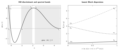
Two equivalent encodings of the $q=1$ Mathieu spectrum. On the left, gray intervals satisfy $|\Delta(a,1)|\leq2$; the white intervals are gaps. On the right, the lowest three fiber eigenvalues sweep those same bands as $0\leq\nu\leq1$. Periodic edges lie at $\nu=0$, antiperiodic edges at $\nu=1$.

The default run gives the empirical audit

Diagnostic	Maximum
Fourier cutoff shift	$8.67\times10^{-13}$
Edge residual $	\Delta\mp2
Wronskian defect $	\det M-1
Symmetry defect $	C(\pi)-S’(\pi)
Monodromy step shift	$3.53\times10^{-11}$

The high mode increases the Fourier cutoff, propagation mesh, and number of bands. Agreement of the printed digits with both refinements is strong floating-point evidence, not a proof that the digits form rigorous intervals. At high index the factorially narrow gaps rapidly approach roundoff; monodromy root finding then becomes ill-conditioned even though the surrounding broad bands remain easy to resolve.

Run the reproducible checks with

python3 public/code/advanced-ode/mathieu-floquet-bands.py
python3 public/code/advanced-ode/mathieu-floquet-bands.py --high \
  --csv /tmp/mathieu-bands.csv
python3 public/code/advanced-ode/mathieu-floquet-bands.py \
  --figure-data /tmp/mathieu-discriminant-band-spectrum

The last command exports the discriminant grid, the three plotted Bloch branches, and the edge table as three CSV files. Their values are embedded in the TikZ source so that the figure remains standalone. The propagator’s double-precision audit is calibrated for $0\leq q\leq8$; stronger coupling requires rescaling or higher-precision propagation rather than merely increasing the Fourier cutoff.

The weak-coupling audit at $q=0.05$ compares the first three numerical gap widths with the $n$-hop formula. Their ratios are respectively $0.99996094$, $0.99972238$, and $0.99995117$.

Narrow bands are lattice tunneling amplitudes

For $q\to+\infty$ with fixed level index $j$, the minima of $2q\cos2x$ lie at $x=\pi/2+\pi\mathbb Z$. Expanding about one minimum gives

$$2q\cos(\pi+2\xi) = -2q+4q\xi^2+O(q\xi^4),$$

so the isolated-well levels begin near

$$\varepsilon_j = -2q+(4j+2)\sqrt q+O(1).$$

Weak overlap between neighboring localized states turns each level into a tight-binding band,

$$E_j(\nu;q) \approx \varepsilon_j-2t_j\cos(\pi\nu).$$

Its width is $4|t_j|$. In fact, for each fixed $j$ the standard characteristic values obey

$$\begin{aligned} b_{j+1}(q)-a_j(q) \sim{}& \frac{2^{4j+5}}{j!} \sqrt{\frac{2}{\pi}} q^{j/2+3/4} \ee^{-4\sqrt q}. \end{aligned}$$

This exact leading asymptotic confirms the barrier exponential. The local oscillator expansion alone fixes neither the sign of $t_j$ nor the width’s prefactor and higher corrections; those require normalized connection data. The next page isolates two wells: the lattice band becomes an even–odd doublet, and the same exponentially small hopping amplitude becomes an instanton transseries.

Common pitfalls

Confusing two Hill objects. A Hill determinant is an infinite-matrix spectral determinant; the Hill discriminant is $\operatorname{tr}M$. They can encode related edge conditions, but they are not interchangeable functions.

Calling a band edge a bound state. Periodic and antiperiodic edge functions are bounded generalized eigenfunctions on the line. Repeating a nonzero cell norm over infinitely many cells makes them non-square-integrable.

Equating a repeated multiplier with two eigenvectors. At an open edge, the multiplier $\pm1$ has one eigenline and a Jordan companion. Two bounded solution lines occur only at a closed gap with $M=\pm I$.

Using one inverse-cosine branch globally. The characteristic exponent is defined modulo sign and even integers. Continue the multiplier or quasimomentum branch rather than repeatedly applying a principal $\arccos$ across bands and gaps.

Mixing small coupling with high energy. Fixed-$n$, $q\to0$ perturbation and fixed-$q$, $n\to\infty$ gap asymptotics happen to share a leading formula. Their remainders, proofs, and numerical conditioning are different.

Exercises

1. Intrinsic monodromy data

Prove $\det M(E)=1$. Then show that both a constant change of fundamental frame and a shift of the cell basepoint preserve $\Delta(E)$.

Solution

Liouville’s formula gives

$$\det Y(x,E) = \det Y(0,E) \exp\!\left( \int_0^x\operatorname{tr}A(s,E)\dd s \right)=1,$$

because $\operatorname{tr}A=0$ and $Y(0)=I$. Hence $\det M=1$. Replacing a fundamental matrix by $YC$ changes the coordinate representation of monodromy to $C^{-1}MC$. Periodicity gives $Y(x_0+L)=Y(x_0)M$, so normalization at $x_0$ gives $M_{x_0}=Y(x_0)MY(x_0)^{-1}$. Determinant and trace are invariant under both conjugations.

2. Why a gap contains no full-line eigenstate

For real $E$ with $|\Delta(E)|>2$, classify the multipliers and explain why no nonzero linear combination of the two Bloch solutions lies in $L^2(\mathbb R)$.

Solution

The roots of $\rho^2-\Delta\rho+1=0$ are real, distinct, and reciprocal. Label them so $|\rho_-|<1<|\rho_+|$. The $\rho_-$ solution decays by repeated translation toward $+\infty$ but grows toward $-\infty$; the $\rho_+$ solution does the opposite. Square integrability at $+\infty$ forces the $\rho_+$ coefficient to vanish, while square integrability at $-\infty$ forces the $\rho_-$ coefficient to vanish. Only the zero solution survives.

3. The two kinds of free edge

Derive $M_0(E)$ and use it to compare $E=0$ with $E=(n\pi/L)^2$, $n\geq1$.

Solution

The normalized solutions are $C(x)=\cos(zx)$ and $S(x)=\sin(zx)/z$, with $E=z^2$. Their values and derivatives at $L$ give the displayed $M_0$. At $z=n\pi/L$, $n\geq1$, both off-diagonal entries vanish and the diagonal entries equal $(-1)^n$, so $M_0=(-1)^nI$: the gap is closed. At $z=0$, $S(L)\to L$ and $S'(L)\to1$, while $C'(L)\to0$. Thus $M_0(0)=\bigl(\begin{smallmatrix}1&L\\0&1\end{smallmatrix}\bigr)$, a nontrivial Jordan matrix.

4. The bilateral Mathieu matrix

Derive the Bloch recurrence and prove that translating by $\pi/2$ makes the unlabelled spectrum even in $q$.

Solution

For one Fourier mode, $-\partial_x^2\ee^{\ii(2m+\nu)x}=(2m+\nu)^2 \ee^{\ii(2m+\nu)x}$. Also $2q\cos2x=q(\ee^{2\ii x}+\ee^{-2\ii x})$, which shifts $m$ to $m\pm1$. Equating coefficients gives

$$[(2m+\nu)^2-a]c_m+q(c_{m-1}+c_{m+1})=0.$$

The unitary translation $T_{\pi/2}$ changes $\cos2x$ to $-\cos2x$, so $T_{\pi/2}H_qT_{\pi/2}^{-1}=H_{-q}$. Unitary equivalence preserves the full spectrum and discriminant.

5. Recover the edge dictionary

Use parity at $x=0$ and the multiplier over a full cell to derive the four half-cell boundary conditions in the table. Then recover the first three spectral bands for $q>0$.

Solution

Even functions obey Neumann data at $0$ and odd functions obey Dirichlet data there. Reflection about $\pi/2$, combined with periodicity or antiperiodicity over $\pi$, determines the right endpoint: even periodic $a_{2r}$ states are NN; odd periodic $b_{2r+2}$ states are DD; even antiperiodic $a_{2r+1}$ states are ND; odd antiperiodic $b_{2r+1}$ states are DN. Interlacing and the strict Mathieu ordering give

$$[a_0,b_1]\cup[a_1,b_2]\cup[a_2,b_3]$$

for the first three bands.

6. Open the first two gaps

Derive both effective matrices on this page by eliminating nonresonant Fourier modes. Verify the leading widths of the first two gaps.

Solution

At $n=1$, a single Fourier hop directly connects momenta $+1$ and $-1$, so the off-diagonal element is $q$. Each mode also couples to one nonresonant momentum-$\pm3$ partner, producing the common second-order shift $q^2/(1-9)=-q^2/8$. No two-hop route connects the resonant pair, so the off-diagonal entry has no $q^2$ term. The eigenvalue split is $2q+O(q^3)$.

At $n=2$, the diagonal second-order shift for momentum $+2$ is

$$q^2\left( \frac{1}{4-0}+ \frac{1}{4-16} \right)=\frac{q^2}{6},$$

and the path $+2\to0\to-2$ gives off-diagonal element $q^2/4$. Symmetry gives the same entries for the other basis vector. The eigenvalue shifts are $q^2(1/6\pm1/4)$, namely $-q^2/12$ and $5q^2/12$. Their difference is $q^2/2$.

7. Audit two numerical representations

Run the default and high modes of the companion program. Explain why the cutoff shift, monodromy step shift, edge residual, determinant defect, and reflection-symmetry defect test different failure modes.

Solution

The cutoff shift tests Fourier truncation; the step shift tests propagation discretization. The edge residual compares independent representations by evaluating the propagated discriminant at a Fourier edge. The determinant defect checks Wronskian preservation, while $|C(\pi)-S'(\pi)|$ checks the extra reflection symmetry of the Mathieu potential. A small determinant defect alone cannot validate the energy: a numerical propagator may nearly preserve area while accumulating phase error. Agreement of all five diagnostics is therefore stronger than any one of them.

8. From a band to a doublet

In a nearest-neighbor basis $|\ell\rangle$ localized in the $\ell$th well, derive the tight-binding dispersion. State what additional data exact WKB must supply before the hopping coefficient is numerically determined.

Solution

Let

$$H|\ell\rangle \approx \varepsilon|\ell\rangle -t|\ell+1\rangle -t|\ell-1\rangle.$$

For the Bloch sum $|\theta\rangle=\sum_\ell\ee^{\ii\ell\theta}|\ell\rangle$, translation of the index gives

$$H|\theta\rangle \approx (\varepsilon-2t\cos\theta)|\theta\rangle.$$

Here $\theta=\pi\nu$. Local harmonic data determine $\varepsilon$ but not $t$. Exact WKB must also fix the barrier cycle, normalized Voros symbols, the relevant Stokes chamber and connection matrices, lateral Borel sums on a Stokes direction, and the global Bloch or parity boundary condition. For two wells the phases reduce to even and odd combinations, whose separation is the corresponding doublet splitting.

References

• NIST Digital Library of Mathematical Functions, §28.2, “Definitions and Basic Properties”, for the standard Mathieu equation, Floquet exponent, Fourier recurrence, characteristic values, parity, and ordering.
• NIST Digital Library of Mathematical Functions, §28.5, “Second Solutions”, for Ince’s noncoexistence theorem, and §28.6, “Expansions for Small q”, for the weak-coupling coefficients and gap asymptotics; see also §28.8, “Asymptotic Expansions for Large q” for fixed-index narrow-band widths.
• NIST Digital Library of Mathematical Functions, §28.29, “Hill’s Equation: Definitions and Basic Properties”, for general Hill monodromy, the discriminant, and Floquet solutions.
• G. Floquet, “Sur les équations différentielles linéaires à coefficients périodiques”, Annales scientifiques de l’École Normale Supérieure 12 (1883), 47–88. Original source for Floquet theory.
• W. Magnus and S. Winkler, Hill’s Equation, Interscience, 1966. Classical treatment of discriminants, stability intervals, and edge structure.
• M. S. P. Eastham, The Spectral Theory of Periodic Differential Equations, Scottish Academic Press, 1973. Direct-integral and absolutely-continuous spectral theory.
• J. E. Avron and B. Simon, “The Asymptotics of the Gap in the Mathieu Equation”, Annals of Physics 134 (1981), 76–84. Fixed-coupling high-gap theorem.