Three Controlled Spectral Capstones

Three laboratories now put the book’s main methods under one discipline: freeze the operator and its domain, draw the turning-point passport, identify only the extra structures that really exist, form a boundary spectral function, and compare its zeros with a calculation that does not reuse the same representation.

The result is intentionally asymmetric. Integer Razavy has a finite algebraic calibration but no imported closed all-orders period formula. Modified Mathieu has a complete pure-$SU(2)$ period and Fredholm-determinant dictionary but no polynomial truncation. The pure quartic has a symmetry-folded TBA and an $A_3$ ODE/IM determinant, but those two descriptions share functional-relation data and are not independent numerical experiments. Knowing these differences is the point of the comparison.

We use the established abbreviations QES for quasi-exact solvability, SW/NS for the Seiberg–Witten/Nekrasov–Shatashvili dictionary, TBA for thermodynamic Bethe ansatz, and ODE/IM for the ODE/integrable-model correspondence.

First reading

Read the method map, the three numerical tables, and the final selection algorithm. On a second pass, study the Razavy endpoint normalization, the modified-Mathieu source crosswalk, and the distinction between the two pure-quartic output maps.

Status ledger

Claim	Status and scope
Razavy critical polynomial at $M=4$, $\zeta=1$	Exact finite-dimensional identity for the first four states
Razavy parity boundary functions	Exact spectral functions after a right-recessive normalization is fixed
Razavy Prüfer roots	Numerical propagation of their zero conditions; no determinant amplitude and no Borel–Padé sum of closed quantum periods
Leading Razavy splitting	Leading semiclassical diagnostic for the only subbarrier doublet
Modified-Mathieu exact-WKB ↔ NS periods	Published, normalization-dependent comparison with high-precision numerical evidence in stated chambers
Modified-Mathieu NS Fredholm formula	Model-specific completed determinant for the two-particle Toda/modified-Mathieu problem
Two-instanton modified-Mathieu table	Reproducible truncation study, not a remainder bound
Pure-quartic exact condition and period reconstruction	Published model-specific exact-WKB/TBA construction with the median and lateral prescriptions fixed
Pure-quartic ODE/IM determinant bridge	Exact functional-relation structure in the stated determinant normalization
Printed spectra	Refined floating-point evidence; none of the tables is an interval certificate

Topology chooses the comparison

All three operators are real-line, parity-invariant, confining Sturm–Liouville problems. That common statement does not make their useful coordinates or exact structures interchangeable.

Laboratory	Physical turning points	Extra structure	Primary spectral gate	Distinct audit
Razavy	Four real below the barrier; two real above it	Finite invariant block only when $M/\hbar\in\mathbb N$	Even or odd right-recessive connection coefficient	Finite-difference grid; critical polynomial on the QES slice
Modified Mathieu	Two real points on the physical logarithmic sheet	Pure-$SU(2)$ quantum curve and NS completion	Entire Fredholm determinant or DCHE Wronskian	Real-line grid; WKB–NS period checksum
Pure quartic	Two real and two imaginary points	$\mathbb Z_4$ symmetry, folded TBA, and $A_3$ ODE/IM	Parity-sensitive exact-WKB condition or determinant zero	Parity-block Rayleigh–Ritz matrix

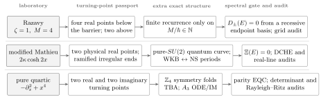
The method is selected after the boundary and turning-point passports are known. A special arithmetic slice, a gauge-theory period dictionary, and a rotational functional relation are three different kinds of additional structure. None follows from the generic phrase “confluent Heun” or “genus one.”

The compact curves reinforce the distinction. With $r=\ee^{2x}$, the Razavy curve is

$$Y^2 = \left[ \zeta(r^2+1)-2Mr \right]^2 -4Er^2.$$

For modified Mathieu, $s=\ee^x$ gives a reciprocal quartic. For the pure quartic, the four roots of $q^4=E$ form a rotational orbit. All three generic compactifications have genus one, but genus alone does not supply a boundary condition, a cycle orientation, a Stokes chamber, or an integral equation.

Capstone A: Razavy across a separatrix

Fix the operator

$$H_{mathrm R} = -\frac{\dd^2}{\dd x^2} +\left(\cosh2x-4\right)^2$$

on $L^2(\mathbb R)$. Its minima are zero and its central barrier has height $V(0)=9$. The $M=4$ recurrence closes and gives

$$\begin{aligned} \Pi_4(E) &= (E-6)(E-14) \left[(E-14)^2-48\right], \\ \{E_0,E_1,E_2,E_3\} &= \left\{ 6, 14-4\sqrt3, 14, 14+4\sqrt3 \right\}. \end{aligned}$$

Parity alternates even, odd, even, odd. Only $E_0$ and $E_1$ lie below the barrier. Thus one critical polynomial crosses a turning-point transition: the first two roots belong to the four-real-turning-point chamber, while the next two belong to the above-barrier two-real-turning-point problem. A single unlabelled double-well quantization formula cannot cover all four roots.

Recessive endpoint data define the boundary functions

Temporarily restore general $\zeta>0$ and $M>0$ in the endpoint formulas. Let $\psi_R(x;E)$ be the solution recessive at the right irregular end. Its canonical asymptotic branch begins

$$\begin{aligned} \psi_R(x;E) \sim{}& \exp\!\left[ -\frac{\zeta}{2}\cosh2x +(M-1)x \right] \left[1+O(\ee^{-2x})\right], \\ \frac{\psi_R'}{\psi_R} ={}& (M-1)-\zeta\sinh2x \\ &- \frac{\zeta^2+2M-1-E}{\zeta} \ee^{-2x} +O(\ee^{-4x}). \end{aligned}$$

The asymptotic condition at infinity defines a canonical recessive line, up to one nonzero normalization. Under the meromorphic exact-WKB hypotheses of Chapter 9, Borel-summed WKB solutions give a sectorial realization and continuation of that line. The numerical lane below instead imposes the displayed endpoint expansion at a finite cutoff and propagates the exact ODE. Reflection reduces the full-line spectral condition to two midpoint connection coefficients:

$$\begin{aligned} D_{\mathrm{even}}(E) &=\psi_R'(0;E), \\ D_{\mathrm{odd}}(E) &=\psi_R(0;E). \end{aligned}$$

Their alternating real zeros are the complete spectrum, including the nonalgebraic states. On the QES slice, define the parity factors

$$\begin{aligned} \Pi_{4,\mathrm{even}}(E) &=(E-6)(E-14), \\ \Pi_{4,\mathrm{odd}}(E) &=(E-14)^2-48. \end{aligned}$$

Locally near the four simple algebraic roots, $D_p=U_p\Pi_{4,p}$ with $U_p\ne0$. Equivalently, the full $\Pi_4$ divides $D_{\mathrm{even}}D_{\mathrm{odd}}$ locally; it does not divide each parity determinant separately.

For stable real-energy propagation, write

$$\psi_R=R\sin\theta, \qquad \psi_R'=R\cos\theta.$$

The exact ODE becomes the bounded Prüfer equation

$$\theta' = \cos^2\theta +(E-V)\sin^2\theta.$$

With the unwrapped branch selected at $x_R$ by the right asymptotic, the $n$th level obeys

$$\theta(0;E_n) = \frac{1-n}{2}\pi.$$

Even $n$ makes $\cos\theta(0)=0$ and hence $D_{\mathrm{even}}=0$; odd $n$ makes $\sin\theta(0)=0$ and hence $D_{\mathrm{odd}}=0$. The angle is a stable real-axis coordinate for finding the zeros. Analyticity in complex $E$ belongs to the Wronskians themselves, not to a globally unwrapped Prüfer phase.

The companion program razavy-wkb-connection.py uses the displayed two-term endpoint expansion, DOP853 propagation, node-aware root brackets, and a second endpoint cutoff:

python3 public/code/advanced-ode/razavy-wkb-connection.py
python3 public/code/advanced-ode/razavy-wkb-connection.py --profile high

Together with the independent finite-difference program from the Razavy page, the high profiles give

$n$	parity	critical polynomial	ODE connection root	coordinate grid
0	even	6.000000000000	6.000000000000	5.999999998836
1	odd	7.071796769724	7.071796769724	7.071796769354
2	even	14.000000000000	14.000000000000	14.000000000543
3	odd	20.928203230276	20.928203230276	20.928203230801
4	even	—	29.863443278037	29.863443278475

The maximum finite-polynomial/connection gap over the algebraic sector is $2.9\times10^{-13}$. Changing the connection initializer from $x_R=2.75$ to $3.5$ moves the five displayed roots by at most $3.1\times10^{-13}$. The coordinate-grid column has a maximum algebraic gap $1.2\times10^{-9}$ and retains much larger pre-extrapolation mesh shifts. Those facts identify three different numerical and algebraic error channels.

What the connection lane does not claim

The connection program locates zeros of the parity boundary functions using the recessive endpoint asymptotic and exact ODE propagation. It does not evaluate their analytic normalization, generate high-order Razavy quantum periods, form Borel transforms, or take lateral Padé sums. Identifying this numerical construction with a summed exact-WKB determinant is conditional on the meromorphic exact-WKB passport. A closed double-well Voros-symbol formula cannot be copied from a polynomial model without auditing the Razavy irregular punctures, cycle orientations, Stokes chamber, and median prescription.

Leading WKB is a diagnostic, not the connection determinant

For the first subbarrier pair, define the right-well and barrier integrals

$$\begin{aligned} I(E) &= \int_{x_{\mathrm{in}}}^{x_{\mathrm{out}}} \sqrt{E-V(x)}\,\dd x, \\ S(E) &= \int_{-x_{\mathrm{in}}}^{x_{\mathrm{in}}} \sqrt{V(x)-E}\,\dd x. \end{aligned}$$

Solving $I(E_c)=\pi/2$ gives

$$\begin{gathered} E_c=6.58614403376377, \qquad S(E_c)=1.09722915254081, \\ I'(E_c)=0.294887454425385. \end{gathered}$$

The leading splitting estimate is therefore

$$\Delta E_{\mathrm{lead}} = \frac{\ee^{-S(E_c)}}{I'(E_c)} =1.13193929647106.$$

The exact algebraic splitting is $8-4\sqrt3=1.07179676972449$, so the leading estimate is $5.61\%$ high. This moderate discrepancy is useful: a leading instanton formula and an exact boundary determinant are not synonyms, even when exact WKB relates both to the same turning-point graph.

For generic sufficiently small $\delta\ne0$, detuning $M=4+\delta$ deletes the $\Pi_4$ lane immediately. Another positive integer $M$ restores a different finite block. The grid and parity determinants survive, and their simple real eigenvalue branches continue analytically. Crossing a Stokes wall reorganizes the WKB coordinates used to represent a determinant; it does not terminate the spectral branch. This negative control is as important as the agreement at $\delta=0$.

Capstone B: modified Mathieu through the NS determinant

Here the special structure is not arithmetic. Begin in the source convention of Grassi–Gu–Mariño:

$$\begin{gathered} \widehat H_{\mathrm s} = -\hbar_{\mathrm s}^2\partial_Q^2 +2\Lambda^2\cosh Q, \\ \widehat H_{\mathrm s}\psi =E_{\mathrm s}\psi, \qquad \psi\in L^2(\mathbb R), \qquad E_{\mathrm s}=2u_{\mathrm s}. \end{gathered}$$

The last equality is the gauge-modulus map, not a choice of units. The flat coordinate below is the energy-dependent quantum mirror map $a_{\mathrm s}=a_{\mathrm s}(E_{\mathrm s},\hbar_{\mathrm s},\Lambda)$. In this passport the exact periods are normalized by

$$\Pi_A^{\mathrm{ex}} =2\pi a_{\mathrm s}, \qquad \Pi_B^{\mathrm{ex}} =2\ii\, \partial_{a_{\mathrm s}}F_{\mathrm{NS}}^{\mathrm s}.$$

At fixed $\Lambda$, the model-specific completed determinant is

$$\Xi_{\mathrm s}(E_{\mathrm s}) = \mathcal N_{\mathrm s}(\hbar_{\mathrm s},\Lambda) \frac{ \cosh\!\left( \Pi_B^{\mathrm{ex}}/(2\hbar_{\mathrm s}) \right) }{ \sinh\!\left( \Pi_A^{\mathrm{ex}}/(2\hbar_{\mathrm s}) \right) },$$

where

$$\mathcal N_{\mathrm s}(\hbar_{\mathrm s},\Lambda) = \frac{ \sinh\!\left( \Pi_A^{\mathrm{ex}}(0)/(2\hbar_{\mathrm s}) \right) }{ \cosh\!\left( \Pi_B^{\mathrm{ex}}(0)/(2\hbar_{\mathrm s}) \right) }$$

fixes $\Xi_{\mathrm s}(0)=1$. Away from a simultaneous denominator zero, the numerator gives

$$\partial_{a_{\mathrm s}} F_{\mathrm{NS}}^{\mathrm s} = \pi\hbar_{\mathrm s} \left(n+\frac12\right).$$

At a simultaneous zero the completed ratio, rather than its numerator, must be evaluated. The operator determinant is entire in $E_{\mathrm s}$, so every apparent pole from the $A$-period denominator or an intermediate Gamma factor must cancel in the full expression. That pole-cancellation requirement is a global check unavailable to a bare period equation.

The source-to-book crosswalk is exact

The Chapter 14 operator is

$$H_\kappa = -\partial_x^2+2\kappa\cosh2x, \qquad H_\kappa\Phi=A\Phi.$$

Putting $Q=2x$ in the source equation and multiplying by $4/\hbar_{\mathrm s}^2$ gives

$$\kappa = \frac{4\Lambda^2}{\hbar_{\mathrm s}^2}, \qquad A = \frac{4E_{\mathrm s}}{\hbar_{\mathrm s}^2}.$$

Thus the Chapter 14 DCHE benchmark $\kappa=4$ fixes the ratio $\Lambda/\hbar_{\mathrm s}=1$. Choosing the unit representative $\Lambda=\hbar_{\mathrm s}=1$ gives $E_{\mathrm s}=A/4$. This algebraic map is safe for the operator. Periods additionally remember the orientation and phase of $\hbar_{\mathrm s}$; a holomorphic Chapter 10 period cannot be continued to the mechanical ray while leaving its Borel direction unchanged.

Exact WKB and NS agree after their analytic prescriptions match

At the off-shell point

$$\Lambda=1, \qquad \hbar_{\mathrm s}=1, \qquad u_{\mathrm s}=4, \qquad E_{\mathrm s}=8,$$

Grassi–Gu–Mariño compared high-order WKB Borel sums with the gauge-resummed periods. Their stabilized values are

Period object	Exact-WKB resummation	NS/gauge resummation
$A$ period	35.40661948105291481767982565	35.40661948105291481767982564492
Reduced $B$ period	16.4748105515008089176353923	16.474810551500808917635392329

The weak $A$ period is ordinarily Borel summable on the stated positive ray. The full weak $B$ period is not; the table removes its non-Borel-summable Gamma/Stirling tail before comparing. For $E_{\mathrm s}>2\Lambda^2$, the published numerical observation compares the restored full period with the arithmetic average of the two lateral WKB sums. No median theorem is inferred from that observation. Summing instantons in $\Lambda^4$ and Borel summing in $\hbar_{\mathrm s}$ remain different analytic operations even where their answers agree.

Two instantons already approach the DCHE spectrum

For readability in the next three displays, suppress the source subscripts: $(a,\hbar,\Lambda)=(a_{\mathrm s},\hbar_{\mathrm s},\Lambda)$. The source NS instanton free energy begins

$$\begin{aligned} F_{\mathrm{NS}}^{\mathrm{inst}} ={}& -\frac{2\Lambda^4}{a^2+\hbar^2} \\ &+ \frac{ \Lambda^8(7\hbar^2-5a^2) }{ (a^2+\hbar^2)^3(a^2+4\hbar^2) } +\cdots, \end{aligned}$$

and

$$\begin{aligned} \partial_aF_{\mathrm{NS}} &=2\gamma(a,\hbar,\Lambda) +\partial_aF_{\mathrm{NS}}^{\mathrm{inst}}, \\ \gamma &= \frac a2\log\frac{\hbar^2}{\Lambda^2} -\frac{\pi\hbar}{4} \\ &\quad- \frac{\ii\hbar}{2} \left[ \log\Gamma\!\left(1+\frac{\ii a}{\hbar}\right) - \log\Gamma\!\left(1-\frac{\ii a}{\hbar}\right) \right]. \end{aligned}$$

After solving the NS condition, the quantum Matone relation supplies the operator energy:

$$E_{\mathrm s} = \frac{a^2}{4} - \frac{\Lambda}{4} \left. \frac{\partial F_{\mathrm{NS}}^{\mathrm{inst}}}{\partial\Lambda} \right|_{a,\hbar}.$$

The companion program modified-mathieu-ns-capstone.py implements these equations through two instantons:

python3 public/code/advanced-ode/modified-mathieu-ns-capstone.py

At $\Lambda=\hbar_{\mathrm s}=1$, the results approach the independently refined DCHE targets from the linked Chapter 14 benchmark monotonically:

$n$	perturbative	one instanton	two instantons	DCHE target
0	2.957944751817	3.057378525702	3.059118455431	3.059174596896
1	5.221650239294	5.284685492053	5.285118923528	5.285125967380
2	7.669023012925	7.714417199922	7.714578100519	7.714579573227
3	10.292571145651	10.327593004583	10.327666526741	10.327666944456

The largest final gap is $5.7\times10^{-5}$, at the ground state. The table shows useful convergence in this parameter regime; it neither bounds the omitted instantons nor replaces the entire Fredholm ratio. The benchmark’s real-line grid and DCHE shooting agree much more closely because both solve the untruncated operator problem.

This capstone therefore closes three different checks:

1. the Borel-summed weak $A$ period and reduced $B$ period agree with their gauge-resummed counterparts off shell in a common analytic passport;
2. the displayed perturbative, one-instanton, and two-instanton NS approximants move successively toward the $L^2$ targets;
3. two boundary-value solvers reproduce the untruncated spectrum directly.

No one of these statements implies a universal SW/NS spectral theorem.

Capstone C: pure quartic through TBA and ODE/IM

Take

$$H_4 = -\frac{\dd^2}{\dd q^2}+q^4$$

on $L^2(\mathbb R)$. The fixed-energy exact-WKB problem

$$\left[-\hbar^2\partial_q^2+q^4-1\right]\psi=0$$

maps to the ordinary spectrum by

$$X=\hbar^{-1}, \qquad \theta=\log X, \qquad E=X^{4/3}.$$

The real and imaginary turning-point pairs carry two independent exact-WKB actions. In the Chapter 13 pure-quartic normalization, the folded two-component TBA reconstructs a median real action $\mathcal A(\theta)$ and a positive complex action $\mathcal B(\theta)$. The parity-sensitive exact condition is

$$\mathcal A(\theta_n) -2(-1)^n \tan^{-1}\!\left( \ee^{-\mathcal B(\theta_n)/2} \right) = 2\pi\left(n+\frac12\right).$$

For the ground state, the nonperturbative correction is about $0.277$ in action units. It is not numerically optional. For $n=3$ it has fallen to about $3.20\times10^{-5}$, displaying how the exact condition approaches its all-orders Bohr–Sommerfeld limit.

Run the complete reconstruction and matrix audit with pure-quartic-tba-spectrum.py:

python3 public/code/advanced-ode/pure-quartic-tba-spectrum.py --high

The first four rows are

$n$	parity	TBA and exact WKB	Rayleigh–Ritz	absolute gap
0	even	1.060362090484179	1.060362090484184	$5.6\times10^{-15}$
1	odd	3.799673029801393	3.799673029801394	$4.4\times10^{-16}$
2	even	7.455697937986746	7.455697937986748	$1.8\times10^{-15}$
3	odd	11.644745511378165	11.644745511378158	$7.1\times10^{-15}$

The digits expose a cross-representation check; they are not a certified continuum error bar. The TBA calculation has separate tail, mesh, fixed-point, principal-value, and root residuals. The Rayleigh–Ritz column varies both its basis size and oscillator frequency.

One TBA solution feeds two model-specific gates

ODE/IM packages the same spectrum into the normalized full-line determinant

$$D_{\mathrm{DT}}(z) = 2\prod_{n=0}^{\infty} \left(1+\frac{z}{E_n}\right), \qquad D_{\mathrm{DT}}(0)=2.$$

Its zeros lie at $z=-E_n$. With $j=\ee^{2\pi\ii/3}$, the determinant obeys

$$\begin{aligned} D_{\mathrm{DT}}(j^{-1}z) D_{\mathrm{DT}}(z) D_{\mathrm{DT}}(jz) ={}& D_{\mathrm{DT}}(j^{-1}z) \\ &+D_{\mathrm{DT}}(z) +D_{\mathrm{DT}}(jz)+2. \end{aligned}$$

At $z=0$, the identity reads $8=2+2+2+2$, which catches a missing full-line normalization immediately. On the positive determinant ray, the TBA output map is

$$\ee^{\varepsilon_1(\theta)} = D_{\mathrm{DT}}\!\left( \ee^{4\theta/3} \right).$$

Analytic continuation and the parity-resolved $Q$ functions reach the physical negative zeros. The real exact-WKB condition instead reconstructs the spectrum directly from $\mathcal A$ and $\mathcal B$. These are two model-specific output maps of one common TBA solution, not two statistically independent numerical data sets. The Rayleigh–Ritz matrix is the independent spectrum check; the determinant functional relation is an additional structural gate.

A practical method-selection algorithm

For a new second-order spectral ODE, use the following order.

1. Freeze the operator passport. Record the kinetic coefficient, energy shift, physical contour, Hilbert space, endpoint conditions, parity or Floquet sector, and parameter ranges.
2. Compute the discriminant geometry. Locate turning points and poles, identify real and complex collisions, orient cycles, and mark the Stokes chamber. Near a collision, replace separated-turning-point WKB by a uniform local model.
3. Ask what extra structure is actually present. Test an algebraic invariant space, a complete SW/NS quantum-curve dictionary, rotational functional relations, or a proven integral-equation correspondence. Do not infer one from genus or Heun class.
4. Construct the boundary spectral function. Use a Wronskian, parity determinant, Hill discriminant, Jost function, or Fredholm determinant. Periods become spectral only after this boundary gate is supplied.
5. Choose one efficient primary representation. A finite recurrence is ideal on a QES slice; a period or TBA system is efficient when its full node–cycle dictionary is known; direct connection propagation is the generic fallback.
6. Add a representation-independent audit. Change from recurrence to coordinate space, from an integral equation to a Hamiltonian matrix, or from a transformed Heun equation to the original real line.
7. Refine inside each lane. Vary endpoint cutoffs, basis size, mesh, quadrature, Borel–Padé order, TBA window, and working precision separately. Agreement between lanes cannot diagnose a shared unresolved cutoff.
8. Run a negative control. Detune the QES integer, cross a separatrix, change parity, or approach a known limiting model. The calculation should fail or reorganize exactly where its hypotheses say it will.

The most common method choices can be summarized compactly.

Geometry or structure	Use first	Mandatory second check
Weak stable anharmonic deformation	Perturbative/Borel data or a spectral matrix	Coordinate grid and strong-coupling scaling
Periodic coefficient with a fixed Bloch fiber	Hill discriminant or monodromy matrix	Fourier-fiber diagonalization and direct monodromy
Integer QES slice, requested state inside the finite sector	Critical polynomial or Jacobi block	Full boundary determinant or coordinate solver
Generic two-ended irregular problem	Sectorially normalized Wronskian	Original-variable grid or an independent transformed equation
Two simple real turning points, no special bridge	Exact WKB or direct connection data	Spectral matrix or shooting
Four real turning points below a barrier	Median/lateral exact WKB with tunnelling cycles	Parity-resolved direct spectrum
Coalescing turning points	Uniform Airy, Weber, or higher local model	Direct calculation across the collision
Complete SW/NS dictionary	NS periods plus Matone/accessory and boundary completion	Exact-WKB resummation and a boundary determinant
Proven ODE/IM or TBA map	Functional or integral equations	Direct determinant or Hamiltonian discretization

What counts as two independent checks

Two columns are not independent merely because they print different quantities. The strongest compact evidence record is

$$\begin{gathered} \text{exact identity or theorem} \quad+ \text{numerical realization}, \\ \text{different representation} \quad+ \text{independent refinement path}, \\ \text{positive benchmark} \quad+ \text{negative control}. \end{gathered}$$

For Razavy, recurrence, boundary propagation, and a coordinate grid satisfy that standard, while detuning removes only the recurrence. For modified Mathieu, the WKB–NS period checksum and the grid–DCHE spectrum comparison test different maps; finite instanton order is a visible approximation axis. For the pure quartic, TBA periods and the ODE/IM determinant are related outputs, so the parity-block matrix is indispensable.

The chapter’s exit competence can now be stated operationally: given a new potential, a reader should be able to draw its turning-point graph, select a boundary spectral function, justify every imported correspondence, and produce two checks whose dominant errors are not the same calculation in disguise.

Common pitfalls

Calling WKB-normalized shooting a Borel–Padé period calculation. The Razavy solver initializes a recessive asymptotic endpoint line and then propagates the exact ODE. Its projective coordinate locates the correct connection zeros, but it neither computes determinant amplitudes nor resums a closed-period series.

Using the QES polynomial above or away from its finite sector. At $M=4$ the polynomial gives only four states, even though the operator has infinitely many. At $M=4+\delta$ it loses spectral status entirely.

Dropping the modified-Mathieu factor of four. Under $Q=2x$, $A=4E_{\mathrm s}/\hbar_{\mathrm s}^2$ and $\kappa=4\Lambda^2/\hbar_{\mathrm s}^2$. Importing only the energy number changes the operator.

Treating instanton truncation as an exact determinant. The two-instanton sequence is an informative approximation to the NS data. Entireness and pole cancellation belong to the completed Fredholm ratio.

Counting TBA and ODE/IM as automatically independent. In the pure quartic they share a functional system and a model-specific output dictionary. A Hamiltonian matrix or direct boundary solver supplies the independent lane.

Selecting a method from the equation’s name. “DCHE,” “Mathieu,” and “genus one” do not specify the physical contour, spectral sector, Stokes chamber, or nonperturbative completion.

Exercises

1. Locate the Razavy separatrix inside the algebraic block

For $\zeta=1$, $M=4$, determine which roots of $\Pi_4$ lie below the barrier. Explain why the parity connection determinant remains one valid spectral object across the barrier even though its WKB graph changes.

Solution

The barrier is $(M-\zeta)^2=9$. The roots $6$ and $14-4\sqrt3\approx7.0718$ lie below it; $14$ and $14+4\sqrt3\approx20.9282$ lie above it. The right-recessive solution and its midpoint values continue as analytic boundary data through ordinary energies. What changes at the separatrix is the turning-point collision and hence the useful exact-WKB cycle chart. A nonuniform four-separated-point formula must be replaced by a uniform connection before continuing to the two-point chamber.

2. Derive the Prüfer target

Starting from $\psi=R\sin\theta$ and $\psi'=R\cos\theta$, derive the angle equation. Show that $\theta(0)=(1-n)\pi/2$ alternates between Neumann and Dirichlet conditions.

Solution

The logarithmic derivative is $y=\psi'/\psi=\cot\theta$. Since $\psi''=(V-E)\psi$, it obeys $y'=V-E-y^2$. Differentiating $y=\cot\theta$ and multiplying by $-\sin^2\theta$ gives

$$\theta' = \cos^2\theta+(E-V)\sin^2\theta.$$

For even $n$, $(1-n)\pi/2$ is an odd half-integer multiple of $\pi$, so $\cos\theta(0)=0$ and $\psi'(0)=0$. For odd $n$, it is an integer multiple of $\pi$, so $\sin\theta(0)=0$ and $\psi(0)=0$. The decreasing unwrapped targets also retain the node count.

3. Detune the QES integer

Replace $M=4$ by $M=4+\delta$. Which three Razavy calculations survive, and which one ceases to define spectral values?

Solution

The real-line operator, its parity-resolved grid, and its endpoint-normalized parity connection functions survive. Their simple eigenvalues can be continued in $\delta$. The finite invariant space leaks at its top degree, so $\Pi_4$ is no longer a characteristic polynomial of the operator. Leading WKB actions also survive away from collisions, but their cycles and Stokes chart must be transported.

4. Audit the modified-Mathieu crosswalk

Starting with the source operator, set $Q=2x$ and recover $\kappa$ and $A$. Convert the Chapter 14 DCHE ground value $A_0=12.236698387584$ at $\kappa=4$ to the source energy for $\Lambda=\hbar_{\mathrm s}=1$.

Solution

Because $\partial_Q^2=\tfrac14\partial_x^2$, multiplying the source equation by $4/\hbar_{\mathrm s}^2$ gives

$$-\partial_x^2 +\frac{8\Lambda^2}{\hbar_{\mathrm s}^2}\cosh2x = \frac{4E_{\mathrm s}}{\hbar_{\mathrm s}^2}.$$

Thus $\kappa=4\Lambda^2/\hbar_{\mathrm s}^2$ and $A=4E_{\mathrm s}/\hbar_{\mathrm s}^2$. At unit source parameters, $E_{\mathrm s,0}=A_0/4=3.059174596896$.

5. Read the NS zeros without creating poles

Derive the half-integer NS condition from the numerator of $\Xi_{\mathrm s}$. Why must the denominator still be inspected?

Solution

The zeros of $\cosh z$ occur at $z=\ii\pi(n+1/2)$. With $z=\Pi_B^{\mathrm{ex}}/(2\hbar_{\mathrm s})$ and $\Pi_B^{\mathrm{ex}}=2\ii\partial_aF_{\mathrm{NS}}$, this gives

$$\partial_aF_{\mathrm{NS}} = \pi\hbar_{\mathrm s}\left(n+\frac12\right).$$

If the $A$-period denominator vanishes at the same energy, a numerator zero can cancel it rather than leave a determinant zero. Since the true Fredholm determinant is entire, the order of both zeros in the completed ratio decides the spectral multiplicity.

6. Verify the pure-quartic ground condition

Use $\mathcal A=3.418934503841784$ and $\mathcal B=3.938425611354309$ to evaluate the ground-state correction and check the exact condition.

Solution

The correction is

$$2\tan^{-1}\!\left(\ee^{-\mathcal B/2}\right) =0.277341850251995.$$

Therefore

$$\mathcal A -2\tan^{-1}\!\left(\ee^{-\mathcal B/2}\right) =3.141592653589789,$$

which equals $\pi$ to the displayed numerical accuracy. Omitting the complex cycle would miss the ground quantization by roughly $0.277$ in action units.

7. Design a method passport for a new potential

A real analytic even potential has four separated real turning points for the requested level, no known algebraic sector, and a tunable parameter that can merge the two inner points. Propose a primary method and two checks both away from and near the merger.

Solution

Away from the merger, use a parity-resolved exact-WKB or connection determinant with the well and barrier cycles explicitly oriented. Check its zeros by a coordinate-space solver and refine the two lanes independently. Near the merger, replace the separated inner-point formula by a uniform Weber model matched to the outer regions; continue to use the coordinate solver as one check and compare the uniform result on both sides of the collision as a second. A generic double-well transseries should not be assumed to remain uniform at the collision.

8. Separate a normalization audit from an independent spectrum

Set $z=0$ in the pure-quartic determinant relation. What does the resulting identity test, and why does it not make ODE/IM an independent numerical check of the TBA levels on this page?

Solution

Since $D_{\mathrm{DT}}(0)=2$, the cubic relation gives $2\cdot2\cdot2=2+2+2+2$, or $8=8$. It tests the full-line determinant normalization and the additive constant in the functional relation. The TBA period reconstruction and the ODE/IM determinant map use the same underlying functional system in this example, so their agreement is a structural cross-check rather than independent numerical evidence. The parity-block Rayleigh–Ritz calculation supplies that independent evidence.

References

• M. Razavy, “An Exactly Soluble Schrödinger Equation with a Bistable Potential”, American Journal of Physics 48 (1980), 285–288. Introduces the hyperbolic QES model and its finite low-energy sector.
• F. Finkel, A. González-López, and M. A. Rodríguez, “On the Families of Orthogonal Polynomials Associated to the Razavy Potential”, Journal of Physics A 32 (1999), 6821–6835. Develops the critical polynomial and finite recurrence in the modern QES language.
• E. Delabaere, H. Dillinger, and F. Pham, “Exact Semiclassical Expansions for One-Dimensional Quantum Oscillators”, Journal of Mathematical Physics 38 (1997), 6126–6184. Constructs WKB solutions normalized at infinity and double-well connection symbols; its polynomial examples do not automatically supply a Razavy formula.
• A. Voros, “Exercises in Exact Quantization”, Journal of Physics A 33 (2000), 7423–7450. Relates canonical recessive solutions to half-line Neumann and Dirichlet determinants.
• N. Nikolaev, “Existence and Uniqueness of Exact WKB Solutions for Second-Order Singularly Perturbed Linear ODEs”, Communications in Mathematical Physics 400 (2023), 463–517. Gives precise existence and uniqueness results for exact-WKB solutions under stated trajectory-domain hypotheses.
• A. Grassi, J. Gu, and M. Mariño, “Non-Perturbative Approaches to the Quantum Seiberg–Witten Curve”, JHEP 07 (2020), 106. Sections 2, 4, and 5 fix the modified-Mathieu period normalization, compare WKB and NS resummations, and derive and test the Fredholm determinant used here.
• N. A. Nekrasov and S. L. Shatashvili, “Quantization of Integrable Systems and Four Dimensional Gauge Theories”, in XVIth International Congress on Mathematical Physics (2010), 265–289. Supplies the Toda/NS framework and distinguishes canonical from modified Mathieu spectral realizations.
• K. K. Kozlowski and J. Teschner, “TBA for the Toda Chain”. Derives the Toda quantization conditions from Baxter/TBA data under explicit analytic assumptions.
• K. Ito, M. Mariño, and H. Shu, “TBA Equations and Resurgent Quantum Mechanics”, JHEP 01 (2019), 228. Provides the exact-WKB/TBA period dictionary and the pure-quartic exact condition used in the final capstone.
• P. Dorey and R. Tateo, “Anharmonic Oscillators, the Thermodynamic Bethe Ansatz, and Nonlinear Integral Equations”, Journal of Physics A 32 (1999), L419–L425. Gives the quartic ODE/IM determinant normalization, functional relation, parity map, and benchmark levels.