Entire Spectral Determinants and Canonical Products

A spectral determinant becomes useful for ODE/IM only after two logically different facts have been joined. The ODE must first produce an entire boundary function whose zeros are the spectrum of a declared problem. Its growth must then be controlled strongly enough that the zero divisor can be turned into a canonical product with a fixed zero-free factor.

The Chapter 2 determinant ledger already separates boundary Wronskians, Fredholm determinants, zeta determinants, and canonical products in general. This page specializes that ledger to the confining oscillator family used by ODE/IM and proves when the normalized constructions actually coincide.

For the even homogeneous oscillator

$$H_M = -\frac{\dd^2}{\dd x^2}+x^{2M}, \qquad M\in\mathbb N,$$

these steps meet cleanly. On the half-line, one canonical solution recessive at $+\infty$ produces both the Dirichlet and Neumann determinants. If $M>1$, their order is

$$\rho_M = \frac{M+1}{2M} <1,$$

so their normalized forms are determined by their zeros alone and have genus-zero products. At $M=1$, however, $\rho_M=1$. The same zeros and even the condition $D(0)=1$ leave an exponential $\ee^{cE}$ undetermined. The harmonic oscillator makes that surviving factor completely explicit.

Chapter question

How do global ODE connection identities become functional relations of quantum integrability, and which parts of that passage are ODE theorems rather than integrable-model identifications?

The result to retain

For $M>1$ and $B\in\{\mathrm D,\mathrm N\}$, let $E_n^B$ be the Dirichlet or Neumann half-line eigenvalues. With the recessive solution normalized below,

$$\begin{aligned} D_{\mathrm D}(E) &= \prod_{n=0}^{\infty} \left(1-\frac{E}{E_n^{\mathrm D}}\right), \\ D_{\mathrm N}(E) &= \prod_{n=0}^{\infty} \left(1-\frac{E}{E_n^{\mathrm N}}\right). \end{aligned}$$

The equalities use four inputs: a canonical recessive solution entire in $E$, the boundary-zero characterization, the spectral growth law, and Hadamard factorization. None of them identifies $D_B$ with a Baxter $Q$-function; that extra dictionary is postponed to Page 4.

Status ledger

Statement used on this page	Status
Existence and uniqueness of a sectorially normalized recessive solution, entire in $E$	Classical global ODE theorem for the stated polynomial family and sector
The same assertion for arbitrary real $M>0$	Requires a branch of $x^{2M}$ and the corresponding theorem on the chosen cover; not inferred here from the integer case
Zeros of the endpoint functions equal the declared half-line eigenvalues	Exact boundary-value argument
Positivity, discreteness, and simplicity of those eigenvalues	Self-adjoint separated Sturm–Liouville theorem for the displayed domains
The counting exponent $\rho_M=(M+1)/(2M)$	Weyl asymptotic; the matching upper growth bound for the entire boundary function comes from global ODE analysis
Genus-zero products for $M>1$	Hadamard factorization after the growth estimate and normalization at $E=0$
Equality with an ordinary Fredholm determinant	The determinant exists because $H_{M,B}^{-1}$ is trace class; equality follows from the common genus-zero product and normalization at $E=0$
Equality with a normalized zeta determinant	Comparison theorem for this confining polynomial problem after the zeta continuation and spectral convention are fixed
Harmonic reciprocal-gamma and Hurwitz-zeta formulae	Exact special-function calculations on this page
Identification with a Baxter $Q$-function	Model-dependent and deferred; it requires rotation, Stokes, parameter, and normalization dictionaries

One recessive solution produces two determinants

Work first with an integer $M>1$ and the equation

$$\left[ -\frac{\dd^2}{\dd x^2}+x^{2M} \right]y(x,E) = E\,y(x,E).$$

In the sector containing the positive real axis, global asymptotic ODE theory selects a unique solution $y_0(x,E)$ once its leading coefficient is fixed. We choose

$$y_0(x,E) = x^{-M/2} \exp\left( -\frac{x^{M+1}}{M+1} \right) \left[1+O\!\left(x^{1-M}\right)\right]$$

as $x\to+\infty$, uniformly for $E$ in compact subsets of the energy plane. Multiplying this solution by an $E$-dependent, nowhere-zero entire function would preserve recession but would change every absolute connection coefficient. The printed leading coefficient is therefore part of the definition.

The Sibuya construction gives more than a formal WKB expression: $y_0(x,E)$ and $\partial_x y_0(x,E)$ are entire in $E$ for fixed $x$. Since zero is not an eigenvalue of either half-line problem, define

$$\begin{aligned} D_{\mathrm D}(E) &:= \frac{y_0(0,E)}{y_0(0,0)}, \\ D_{\mathrm N}(E) &:= \frac{\partial_x y_0(0,E)} {\partial_x y_0(0,0)}. \end{aligned}$$

Both functions are entire and equal one at $E=0$. The labels state the endpoint functional rather than an author-dependent sign convention. A common ODE/IM convention calls the Dirichlet or odd determinant $D^-$ and the Neumann or even determinant $D^+$, but the endpoint should always be checked before using a superscript.

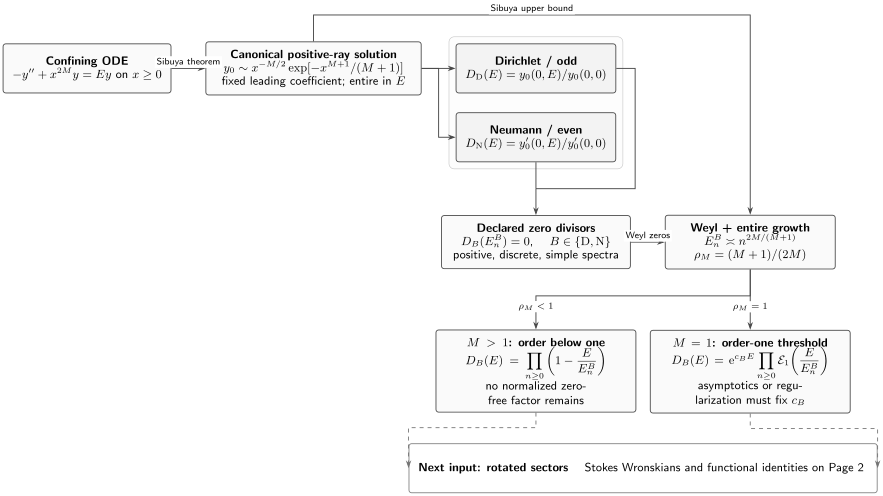
The ODE-to-entire-function pipeline. Canonical normalization at infinity fixes an entire recessive solution; the two endpoint functionals define different half-line spectra. Weyl growth fixes the exponent of convergence and, together with the global ODE growth bound, the order of the entire functions. For $M>1$ the normalized determinants have genus zero. At $M=1$, a zero-free exponential survives and must be fixed by an additional normalization prescription.

What the zeros mean

Let $H_{M,\mathrm D}$ and $H_{M,\mathrm N}$ be the self-adjoint realizations in $L^2(0,\infty)$ with domains

$$\begin{aligned} \mathcal D(H_{M,\mathrm D}) &= \left\{ u\in\mathcal D_{\max}:u(0)=0 \right\}, \\ \mathcal D(H_{M,\mathrm N}) &= \left\{ u\in\mathcal D_{\max}:u'(0)=0 \right\}, \end{aligned}$$

where $\mathcal D_{\max}$ is the maximal operator domain on which $-u''+x^{2M}u$ belongs to $L^2(0,\infty)$. The confining potential makes both resolvents compact. Their spectra are positive, discrete, and simple:

$$0<E_0^B<E_1^B<\cdots, \qquad E_n^B\longrightarrow\infty, \qquad B\in\{\mathrm D,\mathrm N\}.$$

The recessive solution already supplies the $L^2$ condition at infinity. Consequently,

$$\begin{aligned} D_{\mathrm D}(E)=0 &\quad\Longleftrightarrow\quad E\in\sigma(H_{M,\mathrm D}), \\ D_{\mathrm N}(E)=0 &\quad\Longleftrightarrow\quad E\in\sigma(H_{M,\mathrm N}). \end{aligned}$$

This is exact linear ODE reasoning, not an infinite-product definition. A determinant built from two different recessive sectors is a different boundary problem; its Stokes-Wronskian construction begins on Page 2.

The simplicity of the zeros can also be seen without quoting oscillation theory. At an eigenvalue $E_*$, put $z=\partial_Ey_0(\,cdot\,,E_*)$. Differentiating the ODE gives

$$\frac{\dd}{\dd x} W[y_0,z] = -y_0^2.$$

The Wronskian vanishes at infinity, hence

$$W[y_0,z](0) = \int_0^\infty y_0(x,E_*)^2\,\dd x >0.$$

At a Dirichlet eigenvalue this reads $-y_0'(0,E_*)\,\partial_Ey_0(0,E_*)>0$; at a Neumann eigenvalue it reads $y_0(0,E_*)\,\partial_Ey_0'(0,E_*)>0$. The relevant endpoint derivative with respect to $E$ is therefore nonzero.

Weyl growth fixes the exponent of convergence

The positive turning point is

$$x_t(E)=E^{1/(2M)}.$$

Rescaling $x=E^{1/(2M)}t$ in the half-action gives

$$\begin{aligned} \int_0^{x_t(E)} \sqrt{E-x^{2M}}\,\dd x &= I_M E^{\rho_M}, \\ I_M &:= \int_0^1\sqrt{1-t^{2M}}\,\dd t \\ &= \frac{1}{2M} B\!\left(\frac{1}{2M},\frac32\right) \\ &= \frac{ \sqrt\pi\, \Gamma\!\left(1+\frac{1}{2M}\right) }{ 2\Gamma\!\left(\frac32+\frac{1}{2M}\right) }. \end{aligned}$$

The half-line Weyl law is therefore

$$N_B(E) := \#\left\{n:E_n^B\leq E\right\} = \frac{I_M}{\pi}E^{\rho_M}+O(1).$$

For this smooth one-turning-point problem, the endpoint and turning-point phases refine the leading law to

$$\begin{aligned} I_M(E_n^{\mathrm N})^{\rho_M} &= \pi\left(n+\frac14\right)+o(1), \\ I_M(E_n^{\mathrm D})^{\rho_M} &= \pi\left(n+\frac34\right)+o(1). \end{aligned}$$

In particular,

$$E_n^B \asymp n^{1/\rho_M} = n^{2M/(M+1)}.$$

It follows that, for real $s$,

$$\sum_{n=0}^{\infty}(E_n^B)^{-s} \begin{cases} <\infty, & s>\rho_M,\\ =\infty, & s\leq\rho_M. \end{cases}$$

Thus $\rho_M$ is the exponent of convergence of the zero sequence. The Sibuya large-$E$ estimate supplies the matching upper bound for $D_B(E)$, so each boundary determinant has entire-function order exactly $\rho_M$. The spectrum alone supplies the lower bound, but not the upper bound: multiplying by $\exp(\exp E)$ would preserve every zero while destroying finite order.

The genus threshold is also a trace-class threshold

For $M>1$, one has $\rho_M<1$ and hence

$$\sum_{n=0}^{\infty}\frac1{E_n^B}<\infty.$$

The genus-zero product converges locally uniformly. Hadamard factorization permits no nonconstant polynomial in the zero-free exponential of an entire function of order below one. Since $D_B(0)=1$,

$$D_B(E) = \prod_{n=0}^{\infty} \left(1-\frac{E}{E_n^B}\right), \qquad M>1.$$

The same inequality implies that $H_{M,B}^{-1}$ is trace class. Therefore the ordinary Fredholm determinant exists and

$$\begin{aligned} D_B(E) &= \det\nolimits_{\mathrm F} \left(I-EH_{M,B}^{-1}\right) \\ &= \frac{ \det\nolimits_\zeta(H_{M,B}-E) }{ \det\nolimits_\zeta H_{M,B} }. \end{aligned}$$

In the second line, the right-hand side means the entire continuation of the normalized zeta determinant in the $H-E$ sign convention. Its zeros are at $+E_n^B$. A source that instead writes $\det(H+\lambda)$ places the same zeros at $\lambda=-E_n^B$.

This equality is special, not terminological. The determinant notions page states the distinct existence hypotheses in general. Here the spectral growth happens to make the inverse trace class, and the order bound removes the remaining normalized zero-free factor.

For the quartic oscillator, $M=2$ gives

$$\rho_2=\frac34, \qquad E_n^B\asymp n^{4/3}.$$

Thus $\sum_n(E_n^B)^{-1}$ converges, the linear-factor product is legitimate, and no exponential counterterm is available after $D_B(0)=1$. This elementary observation is the entire-function reason the quartic oscillator is such a clean first ODE/IM laboratory.

Even and odd spectra factor through one Wronskian

On the full line, the solution recessive at $+\infty$ is $y_0(x,E)$, while the one recessive at $-\infty$ is $y_0(-x,E)$. With the book’s Wronskian convention,

$$\begin{aligned} W_x[y_0(-x,E),y_0(x,E)]\big|_{x=0} &= 2y_0(0,E)y_0'(0,E). \end{aligned}$$

Normalize this full-line Wronskian by its value at $E=0$. Then

$$D_{\mathrm{full}}(E) = D_{\mathrm N}(E)D_{\mathrm D}(E).$$

The Neumann zeros are the even full-line levels, and the Dirichlet zeros are the odd levels. This exact factorization works because all three functions use the same recessive solution and compatible constants. It is not permission to multiply two arbitrarily normalized determinants or to assume multiplicativity of unrelated absolute zeta determinants.

The harmonic oscillator remembers an exponential

The Chapter 9 Weber benchmark used a full-line reciprocal-gamma determinant to compare a boundary Wronskian with an exact-WKB cycle condition. The new task here is to split that determinant into even and odd half-line sectors and compare the zero-free factors selected by four entire-function normalizations.

At $M=1$, the growth order reaches one and $\sum_n(E_n^B)^{-1}$ diverges. The spectral products need genus one,

$$\mathcal E_1(w) = (1-w)\ee^w,$$

and Hadamard factorization allows a factor $\ee^{cE}$ even after the value at $E=0$ has been fixed. The solvable oscillator shows every constant.

Consider

$$\left[ -\frac{\dd^2}{\dd x^2}+x^2 \right]f(x,E) = E f(x,E),$$

and put

$$\nu=\frac{E-1}{2}, \qquad f(x,E)=D_\nu(\sqrt2x).$$

The parabolic-cylinder function $D_\nu$ is recessive for positive real $x$. Its endpoint values are

$$\begin{aligned} f(0,E) &= \frac{ 2^{(E-1)/4}\sqrt\pi }{ \Gamma\!\left(\frac{3-E}{4}\right) }, \\ f'(0,E) &= -\frac{ 2^{(E+3)/4}\sqrt\pi }{ \Gamma\!\left(\frac{1-E}{4}\right) }. \end{aligned}$$

Introduce

$$a_{\mathrm N}=\frac14, \qquad a_{\mathrm D}=\frac34.$$

The two spectra are

$$E_n^B = 4(n+a_B),$$

namely $E_n^{\mathrm N}=4n+1$ and $E_n^{\mathrm D}=4n+3$. Normalizing the displayed endpoint values at $E=0$ gives

$$B_B(E) = 2^{E/4} \frac{\Gamma(a_B)} {\Gamma(a_B-E/4)}.$$

The letter $B$ emphasizes that this is the boundary function obtained from the particular standard solution $D_\nu(\sqrt2x)$. Its leading asymptotic coefficient depends on $E$, so it is not the same normalization as the radial Sibuya solution commonly used in ODE/IM.

Four normalized functions with one zero set

For either value of $a=a_B$, define the pure genus-one product

$$P_a(E) := \prod_{n=0}^{\infty} \mathcal E_1\!\left( \frac{E}{4(n+a)} \right).$$

The Weierstrass product for the reciprocal gamma function gives

$$\frac{\Gamma(a)}{\Gamma(a-E/4)} = \exp\left[ \frac{\psi(a)}4E \right] P_a(E),$$

where $\psi=\Gamma'/\Gamma$. Three natural determinant normalizations and the bare canonical product can now be compared exactly:

Normalization	Function equal to one at $E=0$	Coefficient $c$ in $\ee^{cE}P_a(E)$
Pure genus-one product	$P_a(E)$	$0$
Common ODE/IM radial Sibuya normalization	$S_a(E)=\Gamma(a)/\Gamma(a-E/4)$	$\psi(a)/4$
Standard $D_\nu(\sqrt2x)$ endpoint normalization	$B_a(E)=2^{E/4}S_a(E)$	$[\psi(a)+\log2]/4$
Zeta ratio for the spectrum $4(n+a)$	$Z_a(E)=4^{E/4}S_a(E)$	$[\psi(a)+\log4]/4$

Every row is entire, has simple zeros at $E=4(n+a)$, and equals one at $E=0$. No two rows are equal unless their zero-free exponential is also matched. This is the order-one obstruction in its most concrete form.

The zeta row follows in two lines. Initially for large $\operatorname{Re}s$,

$$\zeta_{a,E}(s) = \sum_{n=0}^{\infty} [4(n+a)-E]^{-s} = 4^{-s}\zeta_{\mathrm H} \left(s,a-\frac E4\right).$$

Using

$$\begin{aligned} \zeta_{\mathrm H}(0,q) &= \frac12-q, \\ \zeta_{\mathrm H}'(0,q) &= \log\Gamma(q)-\frac12\log(2\pi), \end{aligned}$$

one obtains

$$\frac{ \det\nolimits_\zeta(H_{1,B}-E) }{ \det\nolimits_\zeta H_{1,B} } = 4^{E/4} \frac{\Gamma(a_B)} {\Gamma(a_B-E/4)}.$$

Thus zeta regularization fixes the missing exponential; it does not make that exponential disappear.

A parity check catches mixed normalizations

Using the same standard parabolic-cylinder solution on both half-lines,

$$\begin{aligned} \frac{ W[f(-x,E),f(x,E)] }{ W[f(-x,0),f(x,0)] } &= B_{\mathrm N}(E)B_{\mathrm D}(E) \\ &= \frac{\sqrt\pi} {\Gamma\!\left(\frac{1-E}{2}\right)}. \end{aligned}$$

The gamma duplication formula proves the second equality, and the zeros are the full sequence $E_n=2n+1$. Replacing only one parity factor by its $S$- or $Z$-normalized cousin would introduce a spurious exponential. The check is therefore not merely algebraic: it tests whether the two endpoint determinants share a compatible infinity normalization.

The determinant passport needed by ODE/IM

Before a spectral determinant enters a functional relation, record the following data.

Datum	Choice on this page	Why it matters later
Differential equation	$-y''+x^{2M}y=Ey$	Fixes the sign and scale of the spectral coordinate
Spatial domain	Positive half-line	Distinguishes radial from lateral sector problems
Infinity condition	Canonical solution recessive on the positive ray	Fixes the zero-free normalization up to the stated convention
Endpoint functional	$y(0,E)$ or $y'(0,E)$	Selects Dirichlet/odd or Neumann/even zeros
Spectral sign	$H-E$	Places the zeros at $+E_n$
Entire order	$\rho_M=(M+1)/(2M)$	Determines the available Hadamard polynomial
Product genus	Zero for $M>1$; one at $M=1$	Decides whether linear factors converge
Remaining zero-free factor	Fixed by growth and asymptotic normalization	Must be transported through rotations and functional identities
Integrable-model object	None yet	A Baxter $Q$-function appears only after a model-specific dictionary

Page 2 will add adjacent canonical sectors and their Stokes Wronskians. Page 3 will exploit the covariance of the homogeneous equation under complex rotations. Pages 4–5 will then ask whether the resulting entire functions, asymptotics, and functional identities match a particular integrable model. The ODE identities can be exact even when that final identification remains conditional.

Common pitfalls

Writing a genus-zero product at the harmonic oscillator. The levels grow linearly, so $\sum_nE_n^{-1}$ diverges. Genus-one primary factors or an equivalent regularization are required.

Assuming the zeros and $D(0)=1$ fix an order-one determinant. They do not fix $\ee^{cE}$. One more asymptotic or logarithmic-derivative datum is needed.

Calling an endpoint Wronskian a zeta determinant. It is first an entire boundary function. Equality with a zeta or Fredholm construction is a comparison theorem with operator and normalization hypotheses.

Mixing the signs $H-E$ and $H+\lambda$. The former has zeros at $E=+E_n$; the latter has zeros at $\lambda=-E_n$. A silent substitution reverses every product argument and later every rotation formula.

Multiplying independently normalized parity determinants. Even and odd zero sets combine correctly only after their zero-free factors are made compatible. The full-line Wronskian provides a direct audit.

Exercises

1. Derive the action constant and phase check. Evaluate $I_M$ by a beta-function substitution. Then set $M=1$ and verify that the Neumann and Dirichlet phase shifts reproduce the exact oscillator levels.

Solution

Put $u=t^{2M}$, so

$$\begin{aligned} I_M &= \frac1{2M} \int_0^1 u^{1/(2M)-1}(1-u)^{1/2}\,\dd u \\ &= \frac1{2M} B\!\left(\frac1{2M},\frac32\right). \end{aligned}$$

Using $\Gamma(1+z)=z\Gamma(z)$ and $\Gamma(3/2)=\sqrt\pi/2$ gives the printed gamma ratio. At $M=1$, $I_1=\pi/4$ and $\rho_1=1$, hence

$$E_n^{\mathrm N}=4\left(n+\frac14\right)=4n+1, \qquad E_n^{\mathrm D}=4\left(n+\frac34\right)=4n+3.$$

2. Locate the product and Fredholm thresholds. Prove that $\sum_n(E_n^B)^{-1}$ converges exactly when $M>1$. Explain why the same condition makes $H_{M,B}^{-1}$ trace class.

Solution

Since $E_n^B\asymp n^{2M/(M+1)}$,

$$\sum_n\frac1{E_n^B}$$

has the same convergence behavior as $\sum_n n^{-2M/(M+1)}$. The exponent exceeds one precisely when $2M>M+1$, or $M>1$. The singular values of the positive compact operator $H_{M,B}^{-1}$ are exactly $(E_n^B)^{-1}$, so this summability condition is also the definition of trace class.

3. Prove that the endpoint zeros are simple. Complete the differentiated Wronskian argument separately for the Dirichlet and Neumann cases.

Solution

At $E=E_*$, write $y=y_0(\,cdot\,,E_*)$ and $z=\partial_Ey_0(\,cdot\,,E_*)$. Then

$$(H_M-E_*)z=y, \qquad W[y,z]'=-y^2.$$

Recession at infinity gives $W[y,z](0)=\int_0^\infty y^2\dd x>0$. If $y(0)=0$, then

$$-y'(0)z(0)>0,$$

so $z(0)=\partial_Ey_0(0,E_*)\neq0$. If $y'(0)=0$, then

$$y(0)z'(0)>0,$$

so $z'(0)=\partial_Ey_0'(0,E_*)\neq0$. Therefore the corresponding entire endpoint function has a simple zero.

4. Recover the harmonic genus-one factor. Show that

$$\frac{\Gamma(a)}{\Gamma(a-E/4)} = \ee^{\psi(a)E/4}P_a(E)$$

by comparing logarithmic derivatives at $E=0$ after the zeros and genus have been fixed.

Solution

Both sides have the simple zeros $E=4(n+a)$ and order one. Their ratio is therefore $\ee^{cE+d}$. Both equal one at $E=0$, so $d=0$. Each factor $\mathcal E_1(E/E_n)$ has vanishing logarithmic derivative at zero, while

$$\left. \frac{\dd}{\dd E} \log\frac{\Gamma(a)}{\Gamma(a-E/4)} \right|_{E=0} = \frac14\psi(a).$$

Thus $c=\psi(a)/4$.

5. Derive the zeta normalization. Starting from $\zeta_{a,E}(s)=4^{-s}\zeta_{\mathrm H}(s,a-E/4)$, derive both the absolute determinant and its ratio at $E=0$.

Solution

Set $q=a-E/4$. Then

$$\begin{aligned} -\zeta_{a,E}'(0) &= \log4\,\zeta_{\mathrm H}(0,q) -\zeta_{\mathrm H}'(0,q) \\ &= \left(\frac12-q\right)\log4 -\log\Gamma(q) +\frac12\log(2\pi). \end{aligned}$$

Therefore

$$\det\nolimits_\zeta(H_a-E) = \frac{ \sqrt{2\pi}\,4^{1/2-a+E/4} }{ \Gamma(a-E/4) }.$$

Dividing by the value at $E=0$ gives

$$Z_a(E) = 4^{E/4} \frac{\Gamma(a)}{\Gamma(a-E/4)}.$$

6. Audit the full-line parity factorization. Use the gamma duplication formula to prove

$$B_{\mathrm N}(E)B_{\mathrm D}(E) = \frac{\sqrt\pi}{\Gamma((1-E)/2)}.$$

Then determine the factor introduced if both $B$ functions are replaced by their zeta-normalized counterparts.

Solution

The product of the two boundary functions is

$$2^{E/2} \frac{ \Gamma(1/4)\Gamma(3/4) }{ \Gamma((1-E)/4)\Gamma((3-E)/4) }.$$

Apply

$$\Gamma(z)\Gamma\left(z+\frac12\right) = 2^{1-2z}\sqrt\pi\,\Gamma(2z)$$

to the numerator with $z=1/4$ and the denominator with $z=(1-E)/4$. The powers of two cancel to give the claimed result. Since $Z_a(E)=2^{E/4}B_a(E)$, replacing both parity factors multiplies the full product by $2^{E/2}$.

7. Identify what fails on a resonance sheet. Suppose resonance poles live on a logarithmic cover of the energy plane. Which steps of the genus-zero argument survive, and which require new input?

Solution

A Wronskian of canonically normalized outgoing solutions may still define a local analytic boundary function on a chosen sheet, and its zeros still express linear dependence of the outgoing boundary lines. The self-adjoint positivity and simplicity statements no longer apply. A pole set on a logarithmic cover is not a zero divisor for an entire function of the energy plane, so the displayed Hadamard product, its order, and the ordinary trace-class determinant require a uniformizing coordinate and new growth or operator estimates. None follows from the resonance condition alone.

References

• Y. Sibuya, Global Theory of a Second Order Linear Ordinary Differential Equation with a Polynomial Coefficient, North-Holland Mathematics Studies 18, 1975, for canonical sectorial solutions, their parameter dependence, and polynomial Stokes geometry.
• P.-F. Hsieh and Y. Sibuya, “On the Asymptotic Integration of Second order linear ordinary differential equations with polynomial Coefficients”, Journal of Mathematical Analysis and Applications 16 (1966), 84–103, for the parameter-uniform recessive-solution construction underlying the Sibuya normalization.
• P. Dorey, C. Dunning, and R. Tateo, “The ODE/IM Correspondence”, Journal of Physics A 40 (2007), R205–R283, especially Sections 4.2–4.3 and 5.2 for canonical solutions, radial determinants, growth, and the genus-zero ODE/IM factorization.
• P. Dorey and R. Tateo, “Anharmonic Oscillators, the Thermodynamic Bethe Ansatz, and Nonlinear Integral Equations”, Journal of Physics A 32 (1999), L419–L425, for the historical homogeneous-oscillator correspondence and its original conjectural integrable-model scope.
• A. Voros, “Exact Resolution Method for General 1D Polynomial Schrödinger Equation”, Journal of Physics A 32 (1999), 5993–6007, with corrigendum, 33 (2000), 5783–5784, for polynomial Schrödinger determinants, complex rotations, exact quantization, and the corrected normalization.
• A. Voros, “Exercises in Exact Quantization”, Journal of Physics A 33 (2000), 7423–7450, for zeta normalization, determinant order, and the endpoint identities for canonically normalized recessive solutions.
• F. Gesztesy and K. Kirsten, “On Traces and Modified Fredholm Determinants for Half-Line Schrödinger Operators with Purely Discrete Spectra”, Quarterly of Applied Mathematics 77 (2019), 615–630, for the trace-class versus modified-determinant threshold on half-line Schrödinger operators.
• F. Gesztesy and K. Kirsten, “Effective Computation of Traces, Determinants, and Zeta-Functions for Sturm–Liouville Operators”, Journal of Functional Analysis 276 (2019), 520–562, for direct comparisons among trace, Fredholm-determinant, and zeta-function data.
• NIST Digital Library of Mathematical Functions, parabolic-cylinder equations and endpoint values and Hurwitz-zeta special values and derivatives, for the exact harmonic oscillator audit.
• B. Ya. Levin, Distribution of Zeros of Entire Functions, Translations of Mathematical Monographs 5, AMS, 1964, for exponents of convergence, canonical products, and finite-order Hadamard factorization.