Perron–Kreuser Theory, Pincherle's Theorem, and Continued Fractions

A formal continued fraction is easy to write and dangerous to trust. The substantive question is whether its finite convergents approach a limit and, if they do, which solution of the underlying three-term recurrence that limit selects.

There is a precise answer. Coefficient asymptotics can establish the existence of a minimal line; finite continued fractions are exactly backward recurrence in a ratio chart; and Pincherle’s theorem identifies their limit with that minimal line. A one-sided endpoint problem is then reduced to

$$\begin{aligned} F_0(\lambda) &= \beta_0(\lambda) +\alpha_0(\lambda)R_1^{\min}(\lambda),\\ F_0(\lambda)&=0. \end{aligned}$$

This page proves that chain in the order in which it is logically valid. It also supplies exact and special-function benchmarks, a projective evaluator, and diagnostics that distinguish a converged finite calculation from an infinite-tail theorem.

A convention firewall for the recurrence tail

Keep the house recurrence

$$\alpha_nu_{n+1} +\beta_nu_n +\gamma_nu_{n-1} =0.$$

The interior tail begins at $n=1$. Assume that

$$\alpha_n\gamma_n\neq0$$

there, apart from any explicitly isolated exceptional indices. A one-sided left endpoint has its own row,

$$\alpha_0u_1+\beta_0u_0=0,$$

and is not an invertible recurrence through the fictitious index $-1$.

Use the forward ratio

$$R_n=\frac{u_n}{u_{n-1}}.$$

Dividing the $n$th row by $u_{n-1}$ and solving for $R_n$ gives the backward Riccati map

$$R_n = -\frac{\gamma_n}{ \beta_n+\alpha_nR_{n+1} }.$$

Repeated substitution therefore produces

$$R_k = -\frac{\gamma_k}{ \displaystyle \beta_k - \frac{\alpha_k\gamma_{k+1}}{ \displaystyle \beta_{k+1} - \frac{\alpha_{k+1}\gamma_{k+2}}{ \beta_{k+2}-\cdots } } }.$$

Three conventions are encoded here:

• the numerator at level $n+1$ is $\alpha_n\gamma_{n+1}$, not $\alpha_{n+1}\gamma_n$;
• every nested numerator is subtracted because one minus sign has already been absorbed into the next ratio;
• a displayed infinite nesting is only a formal fraction until its finite convergents are shown to converge.

Minimality on this page always means minimality as $n\to+\infty$. A ratio is only one affine chart on the solution line: $R_n=\infty$ may merely mean $u_{n-1}=0$. Finally, a finite continued-fraction cutoff is a numerical approximant. It is not polynomial termination of the recurrence.

Poincaré–Perron theory separates limiting roots

Normalize an eventually nonsingular tail by dividing through by $\alpha_n$:

$$\begin{aligned} u_{n+1}+a_nu_n+b_nu_{n-1}&=0,\\ a_n&=\frac{\beta_n}{\alpha_n}, & b_n&=\frac{\gamma_n}{\alpha_n}. \end{aligned}$$

Suppose

$$a_n\longrightarrow a, \qquad b_n\longrightarrow b\neq0,$$

and let $r_1,r_2$ be the roots of

$$r^2+ar+b=0.$$

Theorem — Poincaré–Perron, separated-root form. If $|r_1|\neq|r_2|$, there is a basis $u^{(1)},u^{(2)}$ for which

$$\frac{u_{n+1}^{(j)}}{u_n^{(j)}} \longrightarrow r_j, \qquad j=1,2.$$

Poincaré’s conclusion restricts possible consecutive-ratio limits; Perron’s existence theorem supplies solutions realizing the two roots. If $|r_1|<|r_2|$, then $u^{(1)}$ is minimal relative to $u^{(2)}$. Indeed, away from isolated zeros,

$$\frac{ u_n^{(1)}/u_{n-1}^{(1)} }{ u_n^{(2)}/u_{n-1}^{(2)} } \longrightarrow \frac{r_1}{r_2},$$

so the product of these quotient ratios tends to zero geometrically. The theorem, rather than that short comparison, is what establishes the existence of the two ratio limits.

For the exact recurrence

$$u_{n+1}-3u_n+2u_{n-1}=0,$$

the characteristic roots are $1$ and $2$. Thus $m_n=1$ spans the minimal line and $d_n=2^n$ is dominant. This example will shortly audit every sign in the associated fraction.

The distinct-modulus condition matters. If the roots have equal modulus, the leading limiting equation does not select a smaller branch. This is an inconclusive test, not a theorem that no minimal solution exists.

Perron–Kreuser theory reads power-law Newton edges

Constant limits are too restrictive for many special-function recurrences. An operational second-order form of Perron–Kreuser theory begins instead with

$$a_n\sim a\,n^A, \qquad b_n\sim b\,n^B, \qquad ab\neq0.$$

Here $A,B\in\mathbb R$; the coefficient constants $a,b$ may be complex.

The three terms in the normalized recurrence are represented by the Newton points

$$\begin{gathered} P_0=(0,0),\\ P_1=(1,A),\\ P_2=(2,B). \end{gathered}$$

The relevant upper edges encode the powers that can balance when $u_{n+1}/u_n$ has algebraic size.

Theorem — Perron–Kreuser, usable power-law cases.

1. If $A>B/2$, a basis can be chosen with

   $$\begin{aligned} \frac{d_{n+1}}{d_n} &\sim -a\,n^A,\\ \frac{m_{n+1}}{m_n} &\sim -\frac{b}{a}\,n^{B-A}. \end{aligned}$$

   The second line is minimal because $B-A<A$.

2. If $A=B/2$, let $t_1,t_2$ be the roots of

   $$t^2+at+b=0.$$

   When $|t_1|\neq|t_2|$, a basis has ratios asymptotic to $t_jn^A$. The smaller-modulus branch is minimal.

3. If $A<B/2$, the formal outer balance is $t^2+b=0$, whose two roots have equal modulus. The rigorous conclusion supplied at this level is that every nontrivial solution obeys

   $$\limsup_{n\to\infty} \left[ \frac{|u_n|}{(n!)^{B/2}} \right]^{1/n} = |b|^{1/2}.$$

   The theorem does not provide two consecutive-ratio limits or separate a minimal line in this case.

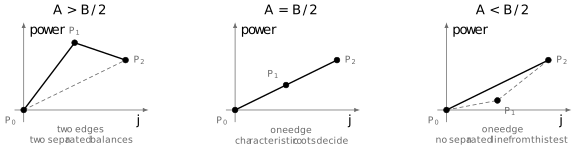
The Newton–Puiseux geometry behind the operational Perron–Kreuser cases. Two edges give two algebraically separated balances; a collinear edge requires the characteristic constants; when the middle point lies below the hull, leading order alone does not select a minimal line.

This theorem is intentionally narrower than the full Newton-polygon theory. Repeated roots, equal-modulus roots, cancellations in subleading coefficients, and transition parameters require a refined analysis. For example,

$$(n+2)u_{n+1} -2(n+1)u_n +nu_{n-1} =0$$

has the exact independent solutions

$$d_n=1, \qquad m_n=\frac{1}{n+1}.$$

After normalization, its limiting characteristic polynomial is $(r-1)^2$. The leading roots coincide, yet $m_n/d_n\to0$. Subleading information discovers a minimal line that the limiting polynomial misses.

The Schwarzschild recurrence derived on the preceding expansion page has the same repeated limiting polynomial. Its refined $n^{-1/2}$ ratio splitting, asymptotic tail seeds, and cutoff-error scale belong to the next page. A numerically stable fraction at one test parameter is useful evidence, but the separated-root theorem alone cannot certify that case.

Finite fractions are projective Miller sweeps

The meaning of the infinite fraction is fixed by its convergents. At depth $N$, impose the canonical terminal ratio

$$R_{N+1}^{[N]}=0$$

and sweep backward:

$$\begin{aligned} R_n^{[N]} &= -\frac{\gamma_n}{ \beta_n+\alpha_nR_{n+1}^{[N]} },\\ n&=N,N-1,\ldots,k. \end{aligned}$$

The first three depths at the fixed head $k$ are

$$R_k^{[k]} = -\frac{\gamma_k}{\beta_k},$$ $$R_k^{[k+1]} = -\frac{\gamma_k}{ \displaystyle \beta_k - \frac{\alpha_k\gamma_{k+1}}{\beta_{k+1}} },$$

and

$$R_k^{[k+2]} = -\frac{\gamma_k}{ \displaystyle \beta_k - \frac{\alpha_k\gamma_{k+1}}{ \displaystyle \beta_{k+1} - \frac{\alpha_{k+1}\gamma_{k+2}}{\beta_{k+2}} } }.$$

Now construct a Miller trial solution $x^{[N]}$ from

$$x_N^{[N]}=1, \qquad x_{N+1}^{[N]}=0,$$

and propagate the recurrence backward. Both $x_n^{[N]}/x_{n-1}^{[N]}$ and $R_n^{[N]}$ obey the same Riccati map and have the same terminal value. Backward induction therefore proves the exact identity

$$R_n^{[N]} = \frac{x_n^{[N]}}{x_{n-1}^{[N]}}.$$

A finite continued fraction, a backward ratio sweep, and a Miller terminal line are not merely analogous algorithms. They are the same projective calculation.

Suppose an actual minimal–dominant basis $m,d$ exists. Write

$$x^{[N]}=A_Nm+B_Nd.$$

The terminal condition at $N+1$ gives

$$\frac{B_N}{A_N} = -\frac{m_{N+1}}{d_{N+1}},$$

whenever the displayed chart is valid. Thus the cutoff error is governed by the minimal–dominant separation. Pincherle’s theorem identifies the limit; it does not promise that a modest cutoff reaches it quickly.

Pincherle identifies the depth limit

Theorem — Pincherle, tail-ratio form. On a nonsingular recurrence tail, the continued fraction headed at $k$ converges to a finite value if and only if the recurrence possesses a minimal solution $m$ with $m_{k-1}\neq0$. In that ratio chart,

$$\lim_{N\to\infty}R_k^{[N]} = \frac{m_k}{m_{k-1}}.$$

Equivalently,

$$\frac{m_k}{m_{k-1}} = -\frac{\gamma_k}{ \displaystyle \beta_k - \frac{\alpha_k\gamma_{k+1}}{ \displaystyle \beta_{k+1} - \frac{\alpha_{k+1}\gamma_{k+2}}{ \beta_{k+2}-\cdots } } }.$$

If $m_{k-1}=0$, the affine value is infinite. The projective statement survives: use homogeneous pairs or switch to the reciprocal ratio. Zeros of an anchor are chart poles, not failures of the recurrence theorem.

Here is the proof in one affine chart. Let $p,q$ be the fundamental solutions normalized by

$$\begin{aligned} p_{k-1}&=1,&p_k&=0,\\ q_{k-1}&=0,&q_k&=1. \end{aligned}$$

A solution with starting ratio $F$ is $p+Fq$. Imposing its finite terminal condition at $N+1$ gives

$$R_k^{[N]} = -\frac{p_{N+1}}{q_{N+1}}.$$

If $R_k^{[N]}\to F$, define $m=p+Fq$. Then

$$\frac{m_{N+1}}{q_{N+1}} = F-R_k^{[N]} \longrightarrow0,$$

so $m$ is minimal relative to the independent solution $q$. Conversely, normalize a minimal solution by $m_{k-1}=1$ and write $m=p+Fq$, where $F=m_k/m_{k-1}$. Minimality relative to $q$ gives $m_n/q_n\to0$, hence $-p_n/q_n\to F$ and the finite convergents approach $F$. Gautschi gives the projective completion through exceptional zero denominators.

Pincherle’s theorem has three important limits:

• it selects a projective line, not an absolute normalization;
• it is an equivalence between fraction convergence and recurrence minimality, not a free proof of either premise in a concrete problem;
• it says nothing by itself about convergence of the original Jaffé, Frobenius, or special-function series at a physical endpoint.

Pointwise convergence in a parameter $\lambda$ also does not automatically give locally uniform convergence or analyticity in $\lambda$. Those properties require uniform tail control away from singular parameter values.

An exact sign and branch-selection test

Return to

$$u_{n+1}-3u_n+2u_{n-1}=0.$$

The backward map is

$$R_n=\frac{2}{3-R_{n+1}}.$$

Starting with $R_{N+1}^{[N]}=0$ gives the exact convergent

$$R_1^{[N]} = \frac{2^{N+1}-2}{2^{N+1}-1} = \frac{1-2^{-N}}{1-2^{-N-1}},$$

and hence

$$R_1^{[N]}-1 = -\frac{2^{-N-1}}{1-2^{-N-1}}.$$

Depth $N$	Exact $R_1^{[N]}$	Error from $1$
$1$	$2/3$	$-1/3$
$2$	$6/7$	$-1/7$
$4$	$30/31$	$-1/31$
$8$	$510/511$	$-1/511$
$12$	$8190/8191$	$-1/8191$

Both $1$ and $2$ are fixed points of the algebraic ratio map, but the continued fraction selects the minimal one. More strongly, for $f(r)=2/(3-r)$,

$$\frac{f(r)-1}{f(r)-2} = \frac12\, \frac{r-1}{r-2}.$$

Every projective terminal line except the exact dominant line therefore converges backward to $1$. An affine denominator may vanish along the way, but the Möbius map itself remains regular on the projective line.

A Bessel benchmark beyond constant coefficients

The cylinder-function recurrence

$$Z_{n+1}(z) -\frac{2n}{z}Z_n(z) +Z_{n-1}(z) =0$$

has independent solutions $J_n(z)$ and $Y_n(z)$. For fixed nonzero $z$, $J_n(z)$ is minimal as the order $n\to+\infty$. At $z=1$, Pincherle’s ratio is

$$\frac{J_1(1)}{J_0(1)} = \frac{1}{ \displaystyle 2 - \frac{1}{ \displaystyle 4 - \frac{1}{ \displaystyle 6 - \frac{1}{8-\cdots} } } }.$$

The finite fractions give:

Depth $N$	Exact convergent	Absolute error
$1$	$1/2$	$7.51\times10^{-2}$
$2$	$4/7$	$3.65\times10^{-3}$
$4$	$180/313$	$1.04\times10^{-6}$
$6$	$21144/36767$	$5.34\times10^{-11}$
$8$	$4686680/8149601$	$8.42\times10^{-16}$

An independent evaluation from the convergent power series gives

$$\begin{aligned} J_0(1) &= 0.76519768655796655145\ldots,\\ J_1(1) &= 0.44005058574493351596\ldots, \end{aligned}$$

and therefore

$$\frac{J_1(1)}{J_0(1)} = 0.57508091500430596050\ldots.$$

By contrast,

$$\frac{Y_1(1)}{Y_0(1)} = -8.8515714113076529710\ldots.$$

The fraction is not just producing some recurrence-compatible ratio; it is selecting the $J$ line. The agreement also audits the nested signs against a special function computed in a completely different representation.

The Leaver residual matches two lines

When $\alpha_0\neq0$, the one-sided endpoint row requires

$$R_1^{\mathrm L} = -\frac{\beta_0}{\alpha_0},$$

while the remote minimal condition requires

$$R_1^{\min} = -\frac{\gamma_1}{ \displaystyle \beta_1 - \frac{\alpha_1\gamma_2}{ \displaystyle \beta_2 - \frac{\alpha_2\gamma_3}{ \beta_3-\cdots } } }.$$

The endpoint and minimal lines coincide exactly when

$$F_0(\lambda) = \beta_0(\lambda) +\alpha_0(\lambda)R_1^{\min}(\lambda) =0.$$

Substituting the fraction gives the one-sided Leaver characteristic residual

$$F_0(\lambda) = \beta_0 - \frac{\alpha_0\gamma_1}{ \displaystyle \beta_1 - \frac{\alpha_1\gamma_2}{ \displaystyle \beta_2-\cdots } }.$$

This is a corollary conditional on existence of the minimal tail and convergence of its continued fraction. It is not legitimate to append an infinite fraction to an arbitrary recurrence and declare the zeros spectral.

Multiplying the endpoint row by a nowhere-zero factor $h(\lambda)$ replaces $F_0$ by $hF_0$. The displayed residual is normalization dependent, while its zero set and zero multiplicities are unchanged wherever $h$ is holomorphic and nonzero.

At a ratio pole, keep the minimal line homogeneous. If $(p,q)=(m_1,m_0)$ represents $R_1=p/q$, use

$$\widehat F_0 = \beta_0q+\alpha_0p.$$

When $q\neq0$, this is $qF_0$; when $q=0$, it remains a regular wedge test between the endpoint and minimal lines.

A deliberately nonspectral algebraic test

For the Schwarzschild recurrence derived earlier, take

$$\varrho=\frac14, \qquad \ell=2, \qquad s=2, \qquad \sigma=3.$$

Its coefficients reduce to

$$\begin{aligned} \mathsf A_n &= (n+1)\left(n+\frac32\right),\\ \mathsf B_n &= -\left(2n^2+4n+\frac92\right),\\ \mathsf C_n &= \left(n-\frac32\right) \left(n+\frac52\right). \end{aligned}$$

The left row fixes

$$\frac{a_1}{a_0}=3.$$

A zero-tail backward sweep has the stable apparent value

$$r_1^{\mathrm{cand}} = -0.17767796980809734549\ldots,$$

with residual

$$\begin{aligned} \mathcal F &= \mathsf B_0+\mathsf A_0r_1^{\mathrm{cand}},\\ \mathcal F &= -4.76651695471214601824\ldots. \end{aligned}$$

Depth $N$	$r_1^{[N]}$
$10$	$-0.1776765305874541$
$20$	$-0.1776779561961947$
$40$	$-0.1776779697758764$
$80$	$-0.1776779698080870$
$160$	$-0.1776779698080973453$

Depth $N$	$\mathcal F_N$
$10$	$-4.766514795881181$
$20$	$-4.766516934294292$
$40$	$-4.766516954663815$
$80$	$-4.766516954712130$
$160$	$-4.7665169547121460180$

The stable nonzero value is the intended numerical result: this algebraic unit test is not a quasinormal mode. It measures a clear mismatch between the left line and the numerically selected remote-line candidate.

What this table establishes

The table shows stable finite-depth arithmetic and decisive disagreement with the left ratio. Because the limiting characteristic root is repeated, the separated-root theorem does not prove infinite-tail convergence here. That missing large-order argument is supplied on the next page.

Split-index residuals expose chart poles

The endpoint residual need not be evaluated at $n=0$. Let $\ell$ be the solution propagated from the left row and $m$ a remote minimal solution. At an interior split $k$, define

$$L_k=\frac{\ell_k}{\ell_{k-1}}, \qquad R_{k+1}=\frac{m_{k+1}}{m_k}.$$

The two half-solutions satisfy the same $k$th recurrence row precisely when

$$F_k = \alpha_kR_{k+1} +\beta_k +\frac{\gamma_k}{L_k} =0.$$

Using the recurrence for $m$ and the Casoratian convention

$$\mathcal K_{k-1}[\ell,m] = \ell_{k-1}m_k-\ell_km_{k-1},$$

one obtains

$$F_k = \gamma_k \frac{ \mathcal K_{k-1}[\ell,m] }{ \ell_km_k }.$$

Every safe split therefore has the same zero set. A pole caused by $\ell_k=0$ or $m_k=0$ is a failure of this scalar chart, not necessarily a singularity of the matched solution. Changing the split or using homogeneous state pairs should recover the same roots, although the conditioning can differ greatly.

This identity is the discrete counterpart of evaluating a boundary Wronskian at different interior points.

Stable evaluation stays projective

Backward homogeneous pairs

Represent a ratio as $R=p/q$. If $(p,q)$ represents $R_{n+1}$, the backward map is

$$(p,q) \longmapsto \left( -\gamma_nq,\, \beta_nq+\alpha_np \right).$$

After every step, divide both $p$ and $q$ by a common scale such as $\max(|p|,|q|)$. This costs $O(N)$ operations and $O(1)$ storage, avoids overflow from growing continuants, and passes through $R=\infty$ without forming the affine ratio.

A practical cutoff test compares projective lines with the chordal distance

$$\begin{aligned} \lVert(p,q)\rVert_2 &= \sqrt{|p|^2+|q|^2},\\ \chi &= \frac{|pQ-Pq|}{ \lVert(p,q)\rVert_2 \lVert(P,Q)\rVert_2 }. \end{aligned}$$

Increase $N$ until the lines agree at two successive depth increments at the requested precision, then repeat at higher working precision and with a second terminal line. A nonzero asymptotic tail seed can accelerate convergence, but it defines a modified approximant whose derivation and error estimate must be supplied.

Modified Lentz as an independent evaluator

For a general continued fraction

$$f = b_0 +\frac{a_1}{ \displaystyle b_1+\frac{a_2}{b_2+\cdots} },$$

the modified Lentz updates are

$$\begin{aligned} D_n&=b_n+a_nD_{n-1}, & D_n&\leftarrow D_n^{-1},\\ C_n&=b_n+\frac{a_n}{C_{n-1}}, & \Delta_n&=C_nD_n,\\ f_n&=f_{n-1}\Delta_n. \end{aligned}$$

Initialize $D_0=0$ and $C_0=f_0=b_0$, replacing an exact or dangerously small divisor by a declared tiny guard. For the Leaver residual,

$$\begin{aligned} b_0&=\beta_0,\\ a_n&=-\alpha_{n-1}\gamma_n, \qquad n\geq1,\\ b_n&=\beta_n. \end{aligned}$$

The tiny replacement is a floating-point guard, not analytic regularization. Likewise, a local test $|\Delta_n-1|<\varepsilon$ is a stopping heuristic, not a proof that the infinite fraction converges. Agreement between Lentz evaluation and a projective backward sweep over increasing depths is a valuable arithmetic cross-check.

Derivatives of finite truncants

For a fixed depth $N$, holomorphic recurrence coefficients make the truncant meromorphic in $\lambda$. On a domain avoiding its poles, differentiate the finite backward sweep. For a zero tail, initialize

$$R_{N+1}^{[N]}=0, \qquad \left(R_{N+1}^{[N]}\right)'=0.$$

For a nonzero tail seed, differentiate that seed instead. In the formulas below, every ratio is the finite-depth quantity $R_n^{[N]}$. Put

$$H_n^{[N]} = \beta_n+\alpha_nR_{n+1}^{[N]}, \qquad R_n^{[N]}=-\frac{\gamma_n}{H_n^{[N]}}.$$

Then

$$\left(H_n^{[N]}\right)' = \beta_n' +\alpha_n'R_{n+1}^{[N]} +\alpha_n\left(R_{n+1}^{[N]}\right)',$$

and

$$\left(R_n^{[N]}\right)' = -\frac{\gamma_n'}{H_n^{[N]}} +\frac{ \gamma_n\left(H_n^{[N]}\right)' }{ \left(H_n^{[N]}\right)^2 }.$$

At the endpoint,

$$\left(F_0^{[N]}\right)' = \beta_0' +\alpha_0'R_1^{[N]} +\alpha_0\left(R_1^{[N]}\right)'.$$

These formulas give the analytic derivative of the finite residual for complex Newton iteration. They may be passed to the infinite minimal-tail residual only on a pole-free parameter domain where the ratios and their derivative sweeps converge locally uniformly. Pointwise convergence of the fraction is insufficient. A magnitude-normalized residual may be useful for reporting, but absolute values and conjugation destroy holomorphicity and do not belong inside a complex Newton step.

An evidence ledger for continued-fraction roots

Finite truncants are meromorphic functions of $\lambda$. Moving poles and nearby zero–pole pairs can imitate a stable root over a short cutoff range. The following checks answer different questions:

Check	What it tests	What it does not prove
Satisfied separated-case Perron–Kreuser hypotheses	Existence and identity of a separated tail	Refined equal-root behavior
Depth sequence $N,N+\Delta,\ldots$	Stability of finite convergents	Infinite-tail convergence
Increased precision	Control of observed roundoff	Tail truncation control
Two terminal seeds	Attraction toward one projective line	Correct physical endpoint condition
Backward sweep versus Lentz	Independent fraction arithmetic	Minimality of the selected line
Several split indices	Chart and conditioning stability	Certified root count
Small $F_N(\lambda)$	A root of the truncated residual	A root of the infinite residual
Small $\lvert F/F'\rvert$	Local root sensitivity estimate	A rigorous enclosure

For a spectral candidate, track zeros and nearby poles as the depth changes, repeat at higher precision, and verify the result in an independent ODE or connection representation. A recurrence residual alone is not a branch test: both the wanted and unwanted lines satisfy every recurrence row.

Division of labor in the rest of the chapter

The next page derives refined large-order ratios, factorial and stretched-exponential scales, asymptotic tail seeds, and connection amplitudes. The following page treats genuine recurrence termination, finite and Hill determinants, and quasi-exact sectors. Later pages interpret the characteristic residual through Green functions and spectra, then turn the numerical checks into certified or independently verified workflows.

Common pitfalls

Treating formal nesting as convergence. An ellipsis defines a pattern, not a limit. Define finite convergents and invoke a theorem or a controlled tail estimate.

Using Pincherle in a circle. Pincherle equates continued-fraction convergence with existence of a minimal solution. It cannot prove minimality by assuming the fraction converges and then prove convergence by assuming the solution is minimal.

Overreading equal-modulus roots. A repeated or equal-modulus leading root makes the simplest Perron–Kreuser test inconclusive. Subleading powers can still separate two solutions.

Losing an index or sign. In the house convention, the first nested product is $\alpha_k\gamma_{k+1}$ and it is subtracted from the next denominator. Re-derive the Riccati map whenever a source uses a different recurrence sign convention.

Calling a cutoff “termination.” Setting $R_{N+1}=0$ defines a finite approximant. Polynomial termination is an exact parameter-dependent decoupling of the infinite recurrence.

Interpreting a ratio pole physically. A vanishing denominator of $u_n/u_{n-1}$ often calls only for a reciprocal or homogeneous chart. Check the projective state before diagnosing divergence.

Accepting a root of one truncant. A root of $F_N$ can drift, collide with a pole, or disappear. Track depth, precision, terminal seed, nearby poles, and preferably more than one split index.

Equating coefficient minimality with endpoint admissibility. Whether a minimal coefficient sequence yields the desired physical solution depends on convergence and analytic continuation of the basis series.

Exercises

1. Derive three convergents

Starting from the house recurrence, derive the backward Riccati map and the first three convergents headed at $k$.

Solution

Divide the $n$th row by $u_{n-1}$:

$$\alpha_nR_{n+1}R_n+\beta_nR_n+\gamma_n=0.$$

Thus

$$R_n = -\frac{\gamma_n}{ \beta_n+\alpha_nR_{n+1} }.$$

At depth $k$, use $R_{k+1}=0$ to obtain $R_k=-\gamma_k/\beta_k$. At depth $k+1$, first compute $R_{k+1}=-\gamma_{k+1}/\beta_{k+1}$ and substitute it into the $k$th map. One more substitution gives

$$R_k^{[k+2]} = -\frac{\gamma_k}{ \displaystyle \beta_k - \frac{\alpha_k\gamma_{k+1}}{ \displaystyle \beta_{k+1} - \frac{\alpha_{k+1}\gamma_{k+2}}{\beta_{k+2}} } }.$$

This establishes both the index shift and the nested minus signs.

2. Evaluate the exact periodic fraction

For

$$u_{n+1}-3u_n+2u_{n-1}=0,$$

prove the formula for $R_1^{[N]}$ and identify its limit.

Solution

The terminal solution satisfying $x_N=1$ and $x_{N+1}=0$ has the form $A+B2^n$. Solving the two terminal equations gives, up to a common nonzero factor,

$$x_n=2^{N+1}-2^n.$$

Therefore

$$R_1^{[N]} = \frac{x_1}{x_0} = \frac{2^{N+1}-2}{2^{N+1}-1}.$$

It tends to $1$, the ratio of the minimal solution $m_n=1$, rather than to $2$, the ratio of the dominant solution.

3. Map a theorem-silent boundary

For real $\lambda\geq0$, compare the recurrence

$$u_{n+1}-2\lambda u_n+u_{n-1} =0$$

in the regimes $\lambda>1$, $\lambda=1$, and $0\leq\lambda<1$. Determine when the separated-root theorem applies and whether a minimal line exists.

Solution

The characteristic roots are

$$r_\pm = \lambda\pm\sqrt{\lambda^2-1}.$$

For $\lambda>1$, they are positive, reciprocal, and have distinct moduli. The line $r_-^n$ is minimal relative to $r_+^n$, so Poincaré–Perron applies directly.

At $\lambda=1$, the root is repeated. A basis is

$$u_n^{(1)}=1, \qquad u_n^{(2)}=n.$$

The constant solution is minimal relative to $n$, although the separated-root theorem is silent.

For $0\leq\lambda<1$, write $\lambda=\cos\theta$ with $0<\theta\leq\pi/2$. The roots $e^{\pm\ii\theta}$ have equal modulus. Their independent solutions have the same envelope, and no nonzero solution is minimal. Thus failure of the modulus gap can lead either to polynomial separation at $\lambda=1$ or to no minimal line below it.

4. Prove that a convergent is a Miller sweep

Let $x_N=1$, $x_{N+1}=0$, and propagate $x$ backward. Prove that $x_n/x_{n-1}=R_n^{[N]}$ at every index where the affine ratios are defined.

Solution

At the terminal edge,

$$\frac{x_{N+1}}{x_N}=0=R_{N+1}^{[N]}.$$

Assume $x_{n+1}/x_n=R_{n+1}^{[N]}$. The $n$th recurrence row gives

$$\frac{x_n}{x_{n-1}} = -\frac{\gamma_n}{ \beta_n+\alpha_nx_{n+1}/x_n } = R_n^{[N]}.$$

Backward induction completes the proof. If an affine denominator vanishes, the same statement holds for homogeneous pairs on the projective line.

5. Apply the power-law cases

Classify the large-$n$ solutions of

$$u_{n+1}+n^2u_n+nu_{n-1}=0$$

to leading ratio order.

Solution

Here

$$a_n=n^2, \qquad b_n=n,$$

so $A=2$, $B=1$, and $A>B/2$. Perron–Kreuser gives

$$\frac{d_{n+1}}{d_n}\sim-n^2, \qquad \frac{m_{n+1}}{m_n}\sim-\frac1n.$$

Products of the leading ratios suggest scales comparable to $(n!)^2$ and $1/n!$, up to signs and subexponential or algebraic factors. The latter is the minimal line.

6. Derive the endpoint residual

Combine the one-sided endpoint row with Pincherle’s ratio. Then determine what happens when the endpoint row is multiplied by a nonzero scalar.

Solution

The endpoint row requires

$$\frac{u_1}{u_0} = -\frac{\beta_0}{\alpha_0}.$$

Pincherle identifies the remote minimal ratio with

$$R_1^{\min} = -\frac{\gamma_1}{ \displaystyle \beta_1 - \frac{\alpha_1\gamma_2}{\beta_2-\cdots} }.$$

Equality of the two lines is

$$F_0 = \beta_0+\alpha_0R_1^{\min} =0.$$

Multiplying the entire endpoint row by $h\neq0$ multiplies $\alpha_0,\beta_0$, and hence $F_0$, by $h$. The zero set is unchanged.

7. Relate a split residual to the Casoratian

With the definitions in the split-index section, prove

$$F_k = \gamma_k \frac{\mathcal K_{k-1}[\ell,m]}{\ell_km_k}.$$

Solution

The recurrence for $m$ gives

$$\alpha_k\frac{m_{k+1}}{m_k}+\beta_k = -\gamma_k\frac{m_{k-1}}{m_k}.$$

Therefore

$$\begin{aligned} F_k &= \gamma_k \left( \frac{\ell_{k-1}}{\ell_k} -\frac{m_{k-1}}{m_k} \right)\\ &= \gamma_k \frac{ \ell_{k-1}m_k-\ell_km_{k-1} }{ \ell_km_k }. \end{aligned}$$

The numerator is $\mathcal K_{k-1}[\ell,m]$. If either denominator vanishes, use a neighboring split or compare the two homogeneous state pairs directly.

8. Audit the Schwarzschild test point

Using the displayed algebraic coefficients, reproduce the cutoff table. Explain why the computation is strong numerical evidence but not yet a proof of convergence of the infinite fraction.

Solution

Initialize $r_{N+1}=0$ and iterate

$$\begin{aligned} r_n &= -\frac{\mathsf C_n}{ \mathsf B_n+\mathsf A_nr_{n+1} },\\ n&=N,N-1,\ldots,1. \end{aligned}$$

Then compute

$$\mathcal F_N = \mathsf B_0+\mathsf A_0r_1^{[N]}.$$

At depths $20,40,80,160$, this reproduces the digits in the table. The minimal-tail candidate approaches approximately $-0.177678$, while the left row demands $3$, so the lines are unambiguously different.

The test shows cutoff stability, precision stability when repeated in higher precision, and a nonzero endpoint mismatch. It does not by itself prove the $N\to\infty$ limit because the normalized recurrence has a repeated limiting characteristic root. A refined asymptotic construction or an independent convergence theorem is still required.

References

• W. Gautschi, “Computational Aspects of Three-Term Recurrence Relations,” SIAM Review 9 (1967), 24–82, DOI: 10.1137/1009002; author-hosted PDF. Theorems 1.1 and 2.1–2.3 are the principal sources for Pincherle, Poincaré–Perron, and the stated Perron–Kreuser cases.
• NIST Digital Library of Mathematical Functions, §2.9, Difference Equations, for asymptotic bases with distinct and coincident characteristic values.
• NIST Digital Library of Mathematical Functions, §3.6, Linear Difference Equations, for minimal solutions, backward recurrence, Miller’s algorithm, and the Bessel example.
• NIST Digital Library of Mathematical Functions, §3.10, Continued Fractions, for scaled continuants, forward evaluation, and modified Lentz-type algorithms.
• NIST Digital Library of Mathematical Functions, §10.6, Recurrence Relations and Derivatives, and §10.19, Large-Order Asymptotic Expansions, for the cylinder-function recurrence and the minimal $J_n$ branch.
• E. W. Leaver, “An Analytic Representation for the Quasi-Normal Modes of Kerr Black Holes,” Proceedings of the Royal Society A 402 (1985), 285–298, DOI: 10.1098/rspa.1985.0119.
• W. J. Lentz, “Generating Bessel Functions in Mie Scattering Calculations Using Continued Fractions,” Applied Optics 15 (1976), 668–671, DOI: 10.1364/AO.15.000668.
• I. J. Thompson and A. R. Barnett, “Coulomb and Bessel Functions of Complex Arguments and Order,” Journal of Computational Physics 64 (1986), 490–509, DOI: 10.1016/0021-9991(86)90046-X.
• R. Wong and H. Li, “Asymptotic Expansions for Second-Order Linear Difference Equations,” Journal of Computational and Applied Mathematics 41 (1992), 65–94, DOI: 10.1016/0377-0427(92)90239-T.