Two Distinct Singular Loci

Two calculations can become singular for completely different reasons. A local Frobenius recurrence can fail because two ODE exponents differ by an integer. A Virasoro block coefficient can have a pole because its internal Verma-module Gram matrix loses rank at a Kac weight.

Both phenomena can produce poles in intermediate formulas, and both can leave logarithms after a parameter limit. That resemblance is the source of the confusion. Their variables, mathematical mechanisms, and repairs are different. Only after a complete ODE/CFT dictionary has been fixed does it make sense to ask whether the two exceptional sets intersect.

The firewall

For a $(2,1)$ degenerate BPZ probe, keep the following tests on separate lines:

$$\boxed{ \begin{array}{ll} \text{endpoint Frobenius resonance:} & 2b\,a_{\mathrm L,j}\in\mathbb Z, \\ \text{internal Kac degeneracy:} & a_{\mathrm L,int} = \displaystyle \pm\frac{rb+s b^{-1}}2, \quad r,s\in\mathbb Z_{>0}. \end{array} }$$

The first condition uses an external momentum attached to a local ODE endpoint. The second uses the internal momentum of the sewn background block. Equal-looking integers do not make these the same divisor.

Status of the statements

Statement	Status
Integer exponent difference is the Frobenius resonance condition	Exact local ODE statement
Every resonant singularity has a logarithm	False; the finite resonant obstruction may vanish
Kac determinant vanishes at the displayed degenerate weights	Exact representation-theoretic statement
A generic inverse-Gram block chart is meromorphic at internal Kac weights	Exact coefficientwise statement
A fully resummed generic block has no other global singularities	Not asserted here
Every Kac divisor is a pole of every four-point block	False; fusion-polynomial zeros or quotient data can remove a residue
Finite-$b$ BPZ dictionary separating the two loci	Exact
Fixed-label Kac divisors collapse to half-integer internal momentum in the classical limit	Exact asymptotic algebra
Termwise substitution into a singular nonresonant frame or Fourier cell	Invalid in general
Finite result at an intersection	Case dependent; it requires both the ODE and CFT limiting prescriptions

Two reading routes

• Core route. Read the opening comparison, the finite-$b$ firewall, unit-central-charge grid, the decision ledger, and the workflow.
• Technical route. Add the Frobenius obstruction, Kac determinant, exact benchmark, and two limiting-frame sections.

The first route is enough to classify a proposed formula. The second shows how to repair it.

One is local in the ODE variable; the other is a parameter pole

The shortest reliable distinction is to ask what becomes singular.

Question	Frobenius locus	Kac or Zamolodchikov locus
Object	Local solution basis of a differential equation	Internal Verma-module block chart
Variable being expanded	Local coordinate $x=z-z_j$	Sewing coordinate $t$, nome $q$, or an irregular scale
Exceptional datum	Difference of local exponents	Internal conformal weight
Algebraic signal	A zero denominator in the Frobenius recurrence	A zero eigenvalue of a Gram matrix
Possible cancellation	Resonant obstruction vanishes	Residue vanishes or several singular cells cancel
Natural replacement	Levelt or logarithmic local frame	Irreducible quotient, residue recursion, or assembled limiting sum
Monodromy effect	May create a Jordan block at one endpoint	None locally unless the parameter dictionary also enforces resonance

A pole in a parameter is not a singular point in the independent variable. Conversely, a logarithmic local solution does not imply that the internal CFT module is degenerate.

This page reserves Frobenius resonance for the local ODE condition. It does not use the word “resonance” here for poles of a continued resolvent, quasinormal frequencies, or other spectral notions.

Frobenius resonance is detected by one finite recurrence step

Near a regular singular point $x=0$, write

$$y''+p(x)y'+q(x)y=0,$$

with

$$p(x) = \sum_{n=0}^{\infty} p_nx^{n-1}, \qquad q(x) = \sum_{n=0}^{\infty} q_nx^{n-2}.$$

The indicial polynomial is

$$I(\rho) = \rho(\rho-1)+p_0\rho+q_0.$$

For

$$y=x^\rho\sum_{n=0}^{\infty}c_nx^n, \qquad c_0=1,$$

coefficient matching gives

$$\begin{aligned} I(\rho+n)c_n ={}& -\sum_{k=0}^{n-1} \left[ (\rho+k)p_{n-k} +q_{n-k} \right]c_k. \end{aligned}$$

Let the two roots satisfy

$$\rho_+-\rho_-=N, \qquad N\in\mathbb Z_{>0}.$$

For the smaller root, the denominator at $n=N$ is

$$I(\rho_-+N) = I(\rho_+) = 0.$$

The numerator at that one step is the resonant obstruction

$$\mathcal O_N := \sum_{k=0}^{N-1} \left[ (\rho_-+k)p_{N-k} +q_{N-k} \right]c_k.$$

For a positive integer gap, two cases must be distinguished:

1. If $\mathcal O_N\neq0$, the smaller-root pure Frobenius series is obstructed and an independent solution contains a logarithm.
2. If $\mathcal O_N=0$, the resonant step is compatible. A second power-type solution may exist after a free coefficient is fixed.

If instead $N=0$, the roots coincide. There is no positive recurrence step and no quantity $\mathcal O_0$ to test: for a genuine scalar second-order regular singularity, an independent solution necessarily has a logarithmic companion. Thus, for $N>0$, the integer condition locates a resonance divisor but does not by itself decide the logarithmic coefficient.

Levelt form records the missing extension datum

For a first-order Fuchsian system, a Levelt frame has the schematic form

$$Y(x) = U(x)x^D x^L, \qquad U(0)\in GL(2,\mathbb C),$$

where $D$ records integral exponent shifts and $L$ contains the remaining exponent and nilpotent data. If

$$L = \lambda I+\nu E_{12},$$

then

$$x^L = x^\lambda \left( I+\nu E_{12}\Log x \right).$$

The number $\nu$ is not determined by the exponent difference alone. It is the local extension datum detected by the resonant recurrence. When $\nu=0$, the local monodromy can be diagonal even at an integer exponent difference.

The full Frobenius treatment derives the logarithmic normalization and repeated-root cases in detail.

For the standard general-Heun equation used earlier in the chapter, the finite-end exponent differences are

$$\theta_0=2a_0, \qquad \theta_t=2a_t, \qquad \theta_1=2a_1.$$

Consequently,

$$\mathcal R_{j,N} := \left\{ \theta_j=N \right\}, \qquad N\in\mathbb Z,$$

is an endpoint resonance divisor. Whether the point is logarithmic or apparent still depends on the relevant Heun recurrence and accessory parameter.

Kac zeros belong to an internal Gram matrix

Keep the book’s Liouville convention

$$\begin{aligned} Q_{\mathrm L} &= b+b^{-1}, \\ c_{\mathrm{Vir}} &= 1+6Q_{\mathrm L}^2, \\ \Delta^{\mathrm{CFT}} &= \frac{Q_{\mathrm L}^2}{4} -a_{\mathrm L}^2. \end{aligned}$$

For positive integers $r,s$, the Kac weight is

$$\Delta_{r,s}^{\mathrm{CFT}} = \frac{Q_{\mathrm L}^2}{4} - \frac{ \left( rb+s b^{-1} \right)^2 }{4}.$$

At descendant level $M$, the Gram determinant factors as

$$\det G_\Delta^{(M)} = C_M \prod_{\substack{r,s\geq1\\rs\leq M}} \left( \Delta-\Delta_{r,s}^{\mathrm{CFT}} \right)^{p(M-rs)}.$$

Here $p(k)$ is the number of integer partitions of $k$, with $p(0)=1$, and the nonzero prefactor $C_M$ depends on the chosen descendant basis.

The divisor

$$\mathcal K_{r,s} := \left\{ \Delta_{\mathrm{int}} = \Delta_{r,s}^{\mathrm{CFT}} \right\}$$

therefore concerns the internal module used in sewing. A generic four-point coefficient has the form

$$\mathcal V_M = \boldsymbol\gamma_{\mathrm R}^{(M)\mathsf T} \left( G_{\Delta_{\mathrm{int}}}^{(M)} \right)^{-1} \boldsymbol\gamma_{\mathrm L}^{(M)}.$$

It is consequently a rational function of $\Delta_{\mathrm{int}}$ and is meromorphic along Kac divisors. The Chapter 6 quotient construction explains why a degenerate irreducible block is not obtained by blind substitution into this inverse-Gram expression.

Level one shows both the pole and its possible removal

At level one,

$$G_\Delta^{(1)}=2\Delta,$$

and the unit-leading four-point block has

$$\mathcal V(t) = 1+\mathcal V_1t+O(t^2),$$

where

$$\mathcal V_1 = \frac{ \left( \Delta+\Delta_t-\Delta_0 \right) \left( \Delta+\Delta_1-\Delta_\infty \right) }{ 2\Delta }.$$

The $(1,1)$ Kac weight is $\Delta_{1,1}=0$. For generic external weights, $\mathcal V_1$ has a simple pole there. If $\Delta_t=\Delta_0$ or $\Delta_1=\Delta_\infty$, one numerator also vanishes and the residue can disappear.

That cancellation is representation-theoretic. It expresses a three-point fusion zero, not a change in any local ODE exponent. At higher levels the analogous residues factor through fusion polynomials.

Zamolodchikov recursion makes the pole coordinate explicit

After extracting the standard elliptic prefactor, the four-point block can be written schematically as

$$\begin{aligned} H_{\Delta_{\mathrm{int}}}(q) ={}& 1 \\ &+ \sum_{r,s\geq1} \frac{ (16q)^{rs}R_{r,s} }{ \Delta_{\mathrm{int}} -\Delta_{r,s}^{\mathrm{CFT}} } H_{\Delta_{r,s}^{\mathrm{CFT}}+rs}(q). \end{aligned}$$

The residue $R_{r,s}$ contains external fusion polynomials and a normalization factor for the singular vector. This formula displays three facts at once:

• the pole coordinate is the internal weight;
• the pole first contributes at level $rs$;
• special external data can make $R_{r,s}=0$.

Calling every denominator a physical singularity is therefore too strong. The generic Verma-module block is meromorphic. A degenerate irreducible block is instead defined after quotienting the null submodule, and an assembled correlator or tau function can have further cancellations among several meromorphic cells.

The BPZ dictionary keeps the two momentum slots separate

Insert a $(2,1)$ degenerate field with momentum $-b/2$. Near an external field of centered momentum $a_{\mathrm L,j}$, the two BPZ exponents are

$$\lambda_\pm = \frac{bQ_{\mathrm L}}2 \pm b\,a_{\mathrm L,j}.$$

Their difference is

$$\lambda_+-\lambda_- = 2b\,a_{\mathrm L,j}.$$

The exact finite-$b$ conditions are therefore

$$\begin{aligned} \mathcal R_{j,N}^{(2,1)} &: & 2b\,a_{\mathrm L,j} &= N, \\ \mathcal K_{r,s} &: & a_{\mathrm L,int} &= \pm \frac{ rb+s b^{-1} }{2}. \end{aligned}$$

The first equation constrains an external momentum. The second constrains the internal sewing momentum. In the unconstrained block parameter space they are distinct codimension-one divisors, and their generic intersection has codimension two.

For a $(1,2)$ probe, the local exponent difference is instead

$$\frac{2a_{\mathrm L,j}}b.$$

Swapping the probe changes the endpoint resonance test. It does not change which internal Gram matrix is being inverted.

There are three degeneracies in this sentence

The fixed $(2,1)$ probe is degenerate so that a second-order BPZ equation exists. An internal background weight can independently hit a Kac divisor and make a generic block chart singular. The resulting BPZ ODE can independently have a resonant endpoint. These are three statements, not three names for one statement.

A dictionary pulls the loci into one parameter space

Let $\boldsymbol\xi$ denote the parameters of the ODE, physical model, or spectral problem. A declared dictionary is a map

$$\Phi: \boldsymbol\xi \longmapsto \left( c(\boldsymbol\xi), \Delta_{\mathrm{int}}(\boldsymbol\xi), \rho_{j,+}(\boldsymbol\xi), \rho_{j,-}(\boldsymbol\xi), \ldots \right).$$

Only after $\Phi$ is fixed should one define the pulled-back sets

$$\begin{aligned} \mathcal R_{j,N} &= \left\{ \boldsymbol\xi: \rho_{j,+}(\boldsymbol\xi) - \rho_{j,-}(\boldsymbol\xi) =N \right\}, \\ \widetilde{\mathcal K}_{r,s} &= \left\{ \boldsymbol\xi: \Delta_{\mathrm{int}}(\boldsymbol\xi) = \Delta_{r,s} \left( c(\boldsymbol\xi) \right) \right\}. \end{aligned}$$

The meaningful double-exceptional set is

$$\mathcal R_{j,N} \cap \widetilde{\mathcal K}_{r,s}.$$

Before pullback, the two divisors live in different factors of the block parameter space. After pullback they can be disjoint, meet transversely, become tangent, or even share a component because a special boundary condition ties external and internal data together. None of those possibilities follows from the names of the loci.

An internal weight usually describes composite monodromy. Thus a Kac divisor can line up with resonance of $M_0M_t$ without lining up with Frobenius resonance of $M_0$ or $M_t$ separately.

The classical limit preserves the distinction

For a heavy lift, set

$$a_j := \lim_{b\to0} b\,a_{\mathrm L,j}, \qquad a := \lim_{b\to0} b\,a_{\mathrm L,int}.$$

The ODE exponent differences are

$$\theta_j=2a_j.$$

Hence endpoint resonance becomes

$$2a_j\in\mathbb Z.$$

On a fixed Kac divisor,

$$b\,a_{\mathrm L,r,s} = -\frac{ r b^2+s }{2},$$

so

$$b\,a_{\mathrm L,r,s} \longrightarrow -\frac s2.$$

Because the weight depends on $a^2$, the leading classical singular locations occur at

$$2a=\pm s, \qquad s\in\mathbb Z_{>0}.$$

Equivalently, with

$$d=\frac14-a^2,$$

the first two fixed-$s$ skeletons are

$$s=1: \quad d=0,$$

and

$$s=2: \quad 4d+3=0.$$

These are the familiar level-one and level-two classical block denominators. They diagnose the internal chart, not an endpoint.

The formulas now look similar:

$$2a_j\in\mathbb Z, \qquad 2a\in\mathbb Z\setminus\{0\}.$$

They still use different coordinates. The first acts on a local endpoint frame; the second acts on the internal block chart selected by the accessory inversion.

There is also a loss of information in the limit. For fixed $s$, all positive $r$ approach the same leading value $a=-s/2$. Subleading $b^2$ data distinguish the finite-$b$ Kac divisors. A classical formula with a pole at $2a=s$ cannot by itself identify the Kac label $r$ or the correct finite-$b$ quotient.

The unit-central-charge grid makes both loci visible

In the $c_{\mathrm{Vir}}=1$ PVI chart, the local exponent lift at zero is $\theta_0$, while the internal composite lift is $\sigma_{0t}$. The endpoint condition is

$$\theta_0\in\mathbb Z.$$

The charge-$n$ internal weight is

$$\Delta_{\mathrm{int},n}^{(1)} = \frac{ \left( \sigma_{0t}+2n \right)^2 }{4}.$$

The $c=1$ Kac lattice is $m^2/4$ with $m\in\mathbb Z$, so the entire charge family meets it exactly when

$$\sigma_{0t}\in\mathbb Z.$$

At $\sigma_{0t}=0$, the $n=0$ primary has $\Delta_{\mathrm{int},0}=\sigma_{0t}^2/4$. A pole that is simple as a function of $\Delta_{\mathrm{int}}$ can therefore look double as a function of $\sigma_{0t}$. This is ramification of the parameter map, not a second null vector. The generic Fourier construction shows which charge–descendant cells must be assembled before taking this limit.

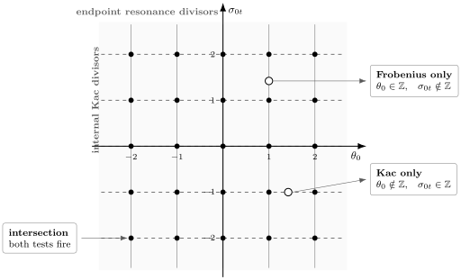
The $c=1$ parameter plane. Vertical lines constrain the local endpoint lift $\theta_0$; horizontal lines constrain the internal composite lift $\sigma_{0t}$. A crossing satisfies two independent conditions.

At $\sigma_{0t}\in\mathbb Z$, the composite trace is

$$\operatorname{tr}(M_0M_t) = 2\cos(\pi\sigma_{0t}) \in \{-2,2\}.$$

This is resonant composite monodromy. It is not local Frobenius resonance at zero unless $\theta_0$ is also an integer.

Three points make the distinction concrete:

$(\theta_0,\sigma_{0t})$	Endpoint zero	Internal channel	Classification
$(1,\sqrt2)$	Resonant	Away from the $c=1$ Kac lattice	Frobenius only
$(\sqrt2,0)$	Nonresonant	Kac-degenerate charge family	Kac only
$(1,0)$	Resonant	Kac-degenerate charge family	Intersection

No change of terminology is needed at the last point. Both diagnoses remain active and both repairs must be performed.

An exact benchmark makes the independence testable

Consider the local ODE family

$$y'' + \frac{1-\vartheta}{x}y' + \left( \frac{\lambda}{x}+\mu \right)y = 0.$$

Its indicial roots at zero are $0$ and $\vartheta$. For the smaller-root series

$$y=\sum_{n=0}^{\infty}a_nx^n, \qquad a_0=1,$$

the recurrence is

$$n(n-\vartheta)a_n + \lambda a_{n-1} + \mu a_{n-2} = 0,$$

where $a_{-1}=a_{-2}=0$. Near the representative resonance $\vartheta=2$,

$$a_1 = \frac{\lambda}{\vartheta-1},$$

and

$$a_2 = \frac{ \lambda^2+\mu(\vartheta-1) }{ 2(\vartheta-2)(\vartheta-1) }.$$

Therefore

$$\lim_{\vartheta\to2} (\vartheta-2)a_2 = \frac{\lambda^2+\mu}{2}.$$

At exact resonance, the compatibility obstruction is

$$\Omega_{\mathrm F} = \lambda^2+\mu.$$

If the larger solution is normalized as $y_2=x^2[1+O(x)]$, the smaller solution has logarithmic coefficient

$$C_{\log} = -\frac{\lambda^2+\mu}{2}.$$

Indeed, the constant term of

$$\mathcal L \left[ 1+\lambda x +C_{\log}y_2\Log x \right]$$

is $\lambda^2+\mu+2C_{\log}$.

The resonance divisor $\vartheta=2$ and the no-log divisor $\mu=-\lambda^2$ are therefore different. On their intersection, for $\lambda\neq0$, two exact analytic solutions are

$$y_0=e^{\lambda x},$$

and

$$y_2 = \frac{ e^{\lambda x} - (1+2\lambda x)e^{-\lambda x} }{ 2\lambda^2 } = x^2+O(x^3).$$

The puncture is apparent: its local monodromy is the identity despite the integer exponent difference. At $\lambda=0$, the displayed $y_2$ has the continuous extension $x^2$, and the pair is simply $(1,x^2)$.

Now attach an independent Virasoro internal weight. Set

$$b^2=2, \qquad c_{\mathrm{Vir}}=28.$$

In the level-two basis $(L_{-2}\lvert\Delta\rangle,L_{-1}^2\lvert\Delta\rangle)$,

$$G_\Delta^{(2)} = \begin{pmatrix} 4\Delta+14&6\Delta\\ 6\Delta&4\Delta(2\Delta+1) \end{pmatrix},$$

so

$$\det G_\Delta^{(2)} = 4\Delta(\Delta+2)(8\Delta+7).$$

The primitive level-two Kac weights are

$$\Delta_{2,1}=-2, \qquad \Delta_{1,2}=-\frac78.$$

For the external weights

$$(\Delta_0,\Delta_t,\Delta_1,\Delta_\infty) = (1,2,3,4),$$

direct inverse-Gram sewing gives

$$\mathcal V_2(\Delta) = \frac{ 2\Delta^4+9\Delta^3+13\Delta^2 +8\Delta-14 }{ 2(\Delta+2)(8\Delta+7) }.$$

Both primitive residues are nonzero:

$$\lim_{\Delta\to-2} (\Delta+2)\mathcal V_2 = 1,$$ $$\lim_{\Delta\to-7/8} \left( \Delta+\frac78 \right)\mathcal V_2 = -\frac{3619}{4096}.$$

The direct-product parameter space therefore contains four decisive points:

Point	$\vartheta$	$(\lambda,\mu)$	$\Delta$	ODE diagnosis	CFT diagnosis
$R$	$2$	$(1,0)$	$1/3$	Resonant and logarithmic	Gram regular
$K$	$3/2$	$(1,0)$	$-2$	Nonresonant	Kac pole
$I$	$2$	$(1,0)$	$-2$	Resonant and logarithmic	Kac pole
$A$	$2$	$(1,-1)$	$-2$	Resonant, log-free, apparent	Kac pole

Point $A$ is the strongest warning: even at an intersection with a Kac pole, endpoint resonance need not produce a logarithm.

The exact benchmark script verifies the recurrence residue, both apparent solutions, the Gram determinant, the block coefficient, and both Kac residues. Run:

python3 public/code/advanced-ode/two-singular-loci-check.py

The audited environment used Python 3.10.16, SymPy 1.13.1, and mpmath 1.3.0. Exact symbolic assertions are followed by residue estimates computed at 70-digit working precision and displayed to 16 significant digits. This benchmark proves logical and computational independence of the two mechanisms. It does not supply an ODE/CFT dictionary between $\vartheta$ and $\Delta$, an all-level block theorem, or a global connection formula.

Similar logarithms can come from different collisions

A local exponent collision

Suppose two normalized solutions depend meromorphically on a parameter $\varepsilon$ and their exponents coalesce:

$$y_-(x;\varepsilon) = x^\rho u(x;0),$$ $$y_+(x;\varepsilon) = x^{\rho+\varepsilon}u(x;\varepsilon),$$

where $u$ is holomorphic in both arguments. Then

$$\lim_{\varepsilon\to0} \frac{ y_+(x;\varepsilon)-y_-(x;\varepsilon) }{\varepsilon} = x^\rho \left[ u(x;0)\Log x +\partial_\varepsilon u(x;0) \right].$$

This logarithm belongs to a local Levelt solution. It changes the endpoint basis and can create a Jordan block in local monodromy.

A collision of meromorphic block cells

Now consider two terms in a tau-function or block-family sum:

$$\begin{aligned} T_\varepsilon(t) ={}& \frac A\varepsilon t^{\kappa+c\varepsilon} \\ &- \frac A\varepsilon t^{\kappa-c\varepsilon}. \end{aligned}$$

On a chosen $\Log t$ branch,

$$T_\varepsilon(t) \longrightarrow 2Ac\,t^\kappa\Log t.$$

Here the logarithm survives only after singular parameter-space cells are assembled. It does not by itself identify a logarithmic endpoint of the auxiliary ODE. In the $c=1$ tau expansion, charge and descendant cells can collide in precisely this way.

The same elementary limit explains the visual similarity, but the objects being recombined are different.

A resonant connection matrix needs a new frame

Let a nonresonant endpoint frame depend on $\varepsilon$:

$$\boldsymbol H_i(\varepsilon) = \left( h_{i,1}(\varepsilon), h_{i,2}(\varepsilon) \right).$$

Suppose a meromorphic matrix $R_i(\varepsilon)$ produces a finite Levelt frame:

$$\boldsymbol H_i^{\mathrm{Lev}} = \lim_{\varepsilon\to0} \boldsymbol H_i(\varepsilon)R_i(\varepsilon).$$

For a simple coalescence, the model recombination is

$$R_i(\varepsilon) = \begin{pmatrix} 1&-\varepsilon^{-1}\\ 0&\varepsilon^{-1} \end{pmatrix},$$

because its second column forms $[h_{i,2}-h_{i,1}]/\varepsilon$. At a nonzero integer difference, the required triangular subtraction is determined by the resonant recurrence rather than this universal model.

If

$$\boldsymbol H_i(\varepsilon) = \boldsymbol H_j(\varepsilon) C_{ji}(\varepsilon),$$

and both endpoints are recombined, then

$$\boxed{ C_{ji}^{\mathrm{Lev}} = \lim_{\varepsilon\to0} R_j(\varepsilon)^{-1} C_{ji}(\varepsilon) R_i(\varepsilon). }$$

Individual entries of $C_{ji}(\varepsilon)$ may diverge while this matrix limit is finite. Substituting $\varepsilon=0$ into gamma functions before applying the two basis changes discards the cancellations.

The Wronskian remains the fastest audit. In the simple coalescing model, $\det R_i\sim\varepsilon^{-1}$ exactly compensates a Wronskian that vanishes like $\varepsilon$.

A Kac limit needs a new block object

The analogous CFT procedure is not an endpoint basis change.

1. Work with generic $\Delta_{\mathrm{int}}$ and identify every pole contributing through the required sewing order.
2. Compute the fusion-polynomial residues. A zero residue can make a nominal Kac pole removable.
3. If the intended internal state is degenerate, replace the Verma module by the appropriate irreducible quotient.
4. If the block occurs inside a Fourier or irregular-state sum, assemble every charge–descendant cell that collides at the retained order.
5. Only then take $\Delta_{\mathrm{int}}\to\Delta_{r,s}$.

The result can be finite, logarithmic in the sewing modulus, or genuinely singular. Which outcome occurs depends on external fusion data and on the larger object being assembled.

At a point lying on both $\mathcal R_{j,N}$ and $\mathcal K_{r,s}$, use both procedures. A safe order is:

$$\begin{gathered} \text{assemble or quotient the generic CFT expression,} \\ \text{derive the corresponding generic ODE relation,} \\ \text{recombine its endpoint frame into Levelt form,} \\ \text{then take the common parameter limit.} \end{gathered}$$

Changing the order is allowed only after uniformity or commutation of the two limits has been proved.

For a genuinely coupled intersection, introduce independent regulators:

$$\rho_{j,+}-\rho_{j,-} = N+\varepsilon_{\mathrm F},$$ $$\Delta_{\mathrm{int}} - \Delta_{r,s} = \varepsilon_{\mathrm K}.$$

Construct the Levelt recombination at generic $\varepsilon_{\mathrm K}$ and assemble the CFT expression at generic $\varepsilon_{\mathrm F}$. Then test the two iterated limits and, when needed, several curves $\varepsilon_{\mathrm K}=c\varepsilon_{\mathrm F}^{\,p}$. A diagonal one-parameter approach can hide path dependence and cannot establish a two-variable limit by itself.

A decision ledger for exceptional formulas

Observed symptom	First diagnostic	Correct action
Frobenius denominator vanishes at step $N$	Compute $\mathcal O_N$	Build a log-free or logarithmic Levelt frame
Gamma entry of a connection matrix diverges as $\theta_j\to N$	Inspect the endpoint basis and Wronskian	Recombine the full matrix on the endpoint side
Gram determinant vanishes at level $rs$	Check $\Delta_{\mathrm{int}}=\Delta_{r,s}$	Compute the fusion residue and specify Verma versus quotient block
One Zamolodchikov residue vanishes	Evaluate the external fusion polynomials	Treat the pole as removable only to the verified order
Individual $c=1$ Fourier cells diverge	Find all cells with the same limiting power	Sum the colliding cells before taking the limit
Accessory inversion reaches $\partial_a q=0$	Test the inverse Jacobian	Change the internal coordinate or use a ramified chart
Both endpoint and internal tests fire	Record both divisors	Apply both limiting prescriptions

The inverse-Jacobian row is a third exceptional set. A branch point of the accessory map is neither a Frobenius resonance nor a Kac divisor, even if all three happen to meet in a special problem.

A reusable intersection workflow

For any proposed ODE/CFT formula:

1. Name the independent parameters. Separate every external momentum, the internal channel momentum, the central-charge parameter, the modulus, and the accessory.
2. Compute each local exponent difference. Mark every integer divisor before using a unit-leading Frobenius frame.
3. Compute the internal Kac weights at finite $b$. Do not infer a Kac label from a classical half-integer alone.
4. Check fusion residues. Decide whether the generic block pole is present, removable, or meaningful only inside an assembled sum.
5. Write the parameter dictionary as a map. Pull both divisors back to the physical or spectral parameter space.
6. Find intersections only after that pullback. Independent divisors can become linked by a boundary condition, symmetry, or minimal-model restriction.
7. Take limits in complete objects. Recombine endpoint frames and assemble block cells before evaluation.
8. Audit the result twice. Use a Wronskian or monodromy test on the ODE side and a quotient, residue, or coefficient test on the CFT side.

Common pitfalls

Calling an integer internal lift “a Frobenius resonance.” An internal composite trace can be resonant while every local endpoint remains nonresonant. State which local loop or composite loop is meant.

Assuming resonance forces a logarithm. The integer exponent difference locates the exceptional recurrence step. The obstruction at that step decides whether a logarithmic coefficient is nonzero.

Calling a Gram zero a pole of the physical theory. The inverse Gram matrix makes a generic Verma-module block meromorphic. Fusion zeros, irreducible quotients, structure constants, or neighboring Fourier cells can remove that pole.

Substituting a resonant value into four separate connection entries. The entries refer to a collapsing nonresonant frame. Apply the full left and right recombination matrices first.

Reading a Kac label from the classical limit. Distinct finite-$b$ divisors with different $r$ can collapse to the same leading half-integer $a$. Preserve the subleading lift whenever the quotient or residue matters.

Exercises

1. Classify three points in the c = 1 plane

Classify

$$(\theta_0,\sigma_{0t}) \in \left\{ (2,\sqrt3), (\sqrt3,-1), (2,-1) \right\}.$$

Solution

At $c=1$, endpoint resonance at zero requires $\theta_0\in\mathbb Z$, whereas the internal Kac family requires $\sigma_{0t}\in\mathbb Z$. Therefore:

• $(2,\sqrt3)$ is Frobenius resonant only;
• $(\sqrt3,-1)$ lies on the internal Kac locus only;
• $(2,-1)$ lies on their intersection.

The final point still requires two separate limiting procedures.

2. Derive the finite-b firewall

Use the $(2,1)$ BPZ exponents

$$\lambda_\pm = \frac{bQ_{\mathrm L}}2 \pm b\,a_{\mathrm L,j}$$

and the centered Kac momentum to derive the two conditions in the opening tip.

Solution

The local exponent difference is

$$\lambda_+-\lambda_- = 2b\,a_{\mathrm L,j}.$$

Frobenius resonance therefore requires this number to be an integer. The Kac formula gives

$$\Delta_{r,s} = \frac{Q_{\mathrm L}^2}{4} - \frac{ (rb+s b^{-1})^2 }{4}.$$

Equating it to $Q_{\mathrm L}^2/4-a_{\mathrm L,int}^2$ gives

$$a_{\mathrm L,int} = \pm \frac{ rb+s b^{-1} }{2}.$$

The two equations constrain different momentum slots.

3. Track a Kac divisor into the classical limit

Fix $r,s$ and show that the leading classical internal momentum loses the label $r$. Explain why this prevents reconstruction of a unique finite-$b$ Kac module.

Solution

For the chosen centered representative,

$$b\,a_{\mathrm L,r,s} = -\frac{ r b^2+s }{2} \longrightarrow -\frac s2.$$

The reflected representative gives $+s/2$. Thus the leading classical location depends on $s$ but not $r$. Every divisor with the same $s$ collapses to the same value. The $O(b^2)$ term $-rb^2/2$ is needed to recover $r$ and hence the finite-$b$ null-vector level $rs$.

4. Test the level-one Kac residue

Find the residue of $\mathcal V_1$ at $\Delta=0$. Give two conditions that make it vanish.

Solution

Multiplying by $\Delta$ and taking the limit gives

$$\operatorname*{Res}_{\Delta=0} \mathcal V_1 = \frac{ (\Delta_t-\Delta_0) (\Delta_1-\Delta_\infty) }{2}.$$

It vanishes if $\Delta_t=\Delta_0$ or if $\Delta_1=\Delta_\infty$. These are fusion zeros. They do not alter the local exponent difference of an unrelated BPZ endpoint.

5. Recover two logarithm mechanisms

Prove the two limits

$$\lim_{\varepsilon\to0} \frac{x^{\rho+\varepsilon}-x^\rho}{\varepsilon},$$

and

$$\lim_{\varepsilon\to0} \frac A\varepsilon \left( t^{\kappa+c\varepsilon} -t^{\kappa-c\varepsilon} \right).$$

Why do identical logarithmic derivatives not identify the underlying singular loci?

Solution

On fixed logarithm branches,

$$x^{\rho+\varepsilon} = x^\rho \left[ 1+\varepsilon\Log x+O(\varepsilon^2) \right],$$

so the first limit is $x^\rho\Log x$. Likewise,

$$t^{\kappa\pm c\varepsilon} = t^\kappa \left[ 1\pm c\varepsilon\Log t+O(\varepsilon^2) \right],$$

and the second limit is $2Ac\,t^\kappa\Log t$. The first recombines two local solutions; the second recombines two meromorphic parameter-space cells. The calculus identity is shared, but the mathematical objects are not.

6. Transform a connection matrix into Levelt frames

Suppose

$$\boldsymbol H_i = \boldsymbol H_jC_{ji}, \qquad \boldsymbol H_\ell^{\mathrm{Lev}} = \lim_{\varepsilon\to0} \boldsymbol H_\ell R_\ell.$$

Derive the Levelt connection matrix and its determinant law.

Solution

Right multiplication gives

$$\begin{aligned} \boldsymbol H_iR_i &= \boldsymbol H_jC_{ji}R_i \\ &= \boldsymbol H_jR_j \left( R_j^{-1}C_{ji}R_i \right). \end{aligned}$$

Therefore

$$C_{ji}^{\mathrm{Lev}} = \lim_{\varepsilon\to0} R_j^{-1}C_{ji}R_i.$$

Before the limit,

$$\det \left( R_j^{-1}C_{ji}R_i \right) = \frac{\det R_i}{\det R_j} \det C_{ji}.$$

This is exactly the Wronskian ratio after changing both endpoint frames. Poles in $\det R_\ell$ compensate zeros in the collapsing nonresonant Wronskians.

References

• NIST Digital Library of Mathematical Functions, §2.7(i), “Regular Singularities: Fuchs–Frobenius Theory”. Gives the indicial equation, coefficient recurrence, and the separate construction required when the indices differ by an integer.
• E. L. Ince, Ordinary Differential Equations, Dover, 1956, Chapter XVI. A classical detailed treatment of regular singular points, exceptional recurrence steps, and logarithmic companions.
• V. G. Kac, “Contravariant Form for Infinite-Dimensional Lie Algebras and Superalgebras”, in Group Theoretical Methods in Physics, Lecture Notes in Physics 94, Springer, 1979, 441–445. Gives the determinant method and irreducibility criterion underlying the Virasoro Kac formula.
• B. L. Feigin and D. B. Fuchs, “Verma Modules over the Virasoro Algebra”, Functional Analysis and Its Applications 17 (1983), 241–242. Describes exceptional Verma-module structure beyond the location of the determinant zeros.
• Al. B. Zamolodchikov, “Conformal Symmetry in Two Dimensions: An Explicit Recurrence Formula for the Conformal Partial Wave Amplitude”, Communications in Mathematical Physics 96 (1984), 419–422. Introduces a recurrence for conformal partial waves from their meromorphic dependence on representation data.
• Al. B. Zamolodchikov, “Conformal Symmetry in Two-Dimensional Space: Recursion Representation of Conformal Block”, Theoretical and Mathematical Physics 73 (1987), 1088–1093. Gives the elliptic recursion in the internal conformal weight.
• M. Cho, S. Collier, and X. Yin, “Recursive Representations of Arbitrary Virasoro Conformal Blocks”, Journal of High Energy Physics 2017 (9), 122. Derives internal-weight and central-charge recursions and makes the factorization of residues into shifted blocks and fusion polynomials explicit.
• O. Gamayun, N. Iorgov, and O. Lisovyy, “Conformal Field Theory of Painlevé VI”, Journal of High Energy Physics 2012 (10), 038; see the erratum. The $c=1$ Fourier-block expansion supplies the concrete charge-cell collision in which internal Kac and composite-monodromy loci meet.
• G. Bonelli, C. Iossa, D. Panea Lichtig, and A. Tanzini, “Irregular Liouville Correlators and Connection Formulae for Heun Functions”, Communications in Mathematical Physics 397 (2023), 635–727. Provides the finite-$b$ degenerate fusion data and the classical Heun dictionaries whose generic formulas require the two separate exceptional-locus tests.

The final page of the chapter turns these distinctions into coefficient recurrences, numerical comparisons, and a status ledger across the Heun confluence hierarchy.