Stage C: Boundary Conditions and Exact Quantization

Page 5 constructed chamber-correct analytic connection coordinates. Those coordinates do not yet select a solution. A spectrum appears only after the left and right admissible solution spaces have been declared and transported into one common frame.

For a scalar second-order problem, each separated endpoint condition usually selects a line in the two-dimensional solution space. The exact quantization function is the determinant of those two transported lines. Its vanishing says that one nonzero solution satisfies both conditions. When exact WKB computes the two lines without approximation, the resulting zero condition is exact as well.

The central result

Let $F_m=(\Psi_{m,+},\Psi_{m,-})$ be a unit-normalized, Borel-summed WKB frame at a matching point, so that $\Wr[\Psi_{m,+},\Psi_{m,-}]=-2/\hbar$. If $T_Lb_L$ and $T_Rb_R$ are the coefficient columns of the left and right admissible solutions in this frame, then

$$\begin{aligned} c_L &:=T_Lb_L, \\ c_R &:=T_Rb_R, \\ \Delta_{\mathrm{WKB}} &:= \det(c_L,c_R) \\ &= -\frac{\hbar}{2} \Wr[\psi_L,\psi_R]. \end{aligned}$$

Thus $\Delta_{\mathrm{WKB}}=0$ is the boundary condition. Calling this formula exact additionally requires the complete analytic passport stated below.

Status ledger

Statement used on this page	Status
Two transported lines meet iff their $2\times2$ determinant vanishes	Exact linear algebra
Determinant–Wronskian identity in a unit WKB frame	Exact once the displayed frame exists
Product of local shears, diagonal transports, sheet exchanges, and monodromy factors	Exact connection algebra for the stated path and conventions
Equality of the WKB product with analytic continuation of exact solutions	Theorem only under summability, geometry, endpoint, and continuation hypotheses
$1+\mathcal V_\gamma=0$ for a one-cycle well	Exact only when the boundary determinant has the stated zero-free factorization
Leading Bohr–Sommerfeld rule	Leading semiclassical consequence, not an exact statement by itself
Weber boundary determinant and spectrum	Exact special-function calculation
Chamber independence of a physical zero divisor	Exact under consistent continuation of frames and boundary lines
A truncated or numerical Borel–Padé evaluation	Approximation to an exact object, with an error still to be assessed

First reading

Follow the boundary-line determinant, the two-turning-point matrix, and the Weber benchmark first. The covariance, Floquet, and multiplicity sections can be read on a second pass.

The ODE is only the first layer of the spectral problem

Retain the book’s Schrödinger convention on a real or complex contour $\mathcal C$, with $V=V(z;\mu,\hbar)$:

$$\left(-\hbar^2\partial_z^2+V\right)\psi =E\psi.$$

and write

$$R:=V-E.$$

Here $E$ is the spectral parameter and $\mu$ denotes fixed couplings. A well-posed spectral claim needs more data than $R$:

$$\mathfrak Q := \left( \begin{gathered} R,\ \mathcal C,\ \arg\hbar,\ L_\theta; \\ \text{graph chamber};\quad \text{cover sheet}; \\ \text{cycle and path basis}; \\ \text{endpoint normalizations}; \\ \mathscr L_L,\ \mathscr L_R;\quad \text{spectral sheet} \end{gathered} \right).$$

The lines $\mathscr L_L$ and $\mathscr L_R$ are the admissible solution spaces at the two ends. The final spectral sheet is redundant for an ordinary self-adjoint bound-state problem, but indispensable for resonances and quasinormal modes.

The spectral-theory interlude explains how the function space and closed operator domain enter. This page does not recreate that operator theory. Its task is to compute the scalar boundary function after the spectral problem has been fixed.

Boundary words select different lines

The phrase “physical solution” must be translated into analytic data.

Boundary word	Actual selection	Extra datum that must be stated
Dirichlet, Neumann, or Robin	Kernel of a finite endpoint covector	Endpoint coordinate and any gauge used to reach normal form
Regular at a regular singular point	A Frobenius line or a specified logarithmic combination	Local exponent, branch, and resonance convention
Recessive or square-integrable	The decaying canonical line in a declared asymptotic sector	Contour end and sector; at thresholds the line can cease to be isolated
Outgoing or ingoing	A canonical oscillatory exponential on a declared sheet	Time dependence, momentum branch, and continuation path
Bloch	An eigenspace of one-period monodromy	Bloch multiplier and period orientation
Coupled system condition	An admissible subspace of the required dimension	Analytic frame or determinant-line convention

For example, “outgoing” changes when the time convention changes from $\ee^{-\ii\omega t}$ to $\ee^{+\ii\omega t}$. It can also change after a square-root branch is crossed. Neither choice is visible in the scalar ODE alone.

Boundary conditions are projective coefficient lines

Let

$$F=(f_+,f_-)$$

be any ordered row frame of exact solutions on a regular overlap. Every solution has a coefficient column

$$\begin{aligned} \psi&=Fc, \\ c&= \begin{pmatrix} c_+\\c_- \end{pmatrix}. \end{aligned}$$

A homogeneous scalar boundary condition is a line, not a normalized vector. If it is written in this frame as

$$\begin{aligned} \ell^{\mathsf T}c&=0, \\ \ell&= \begin{pmatrix} \ell_+\\\ell_- \end{pmatrix}. \end{aligned}$$

then one convenient spanning column is

$$b= \begin{pmatrix} -\ell_-\\\ell_+ \end{pmatrix}.$$

Replacing $b$ by a nonzero scalar multiple does not change the selected solution line. If that scalar depends on $E$, it must be analytic and nowhere zero to preserve the local zero divisor of a boundary function.

Finite-endpoint data can be converted mechanically

At a regular endpoint $z=a$, impose

$$\begin{aligned} 0={}&\alpha_L(E)\psi(a) \\ &+\beta_L(E)\hbar\psi'(a). \end{aligned}$$

For the frame $F=(f_+,f_-)$, define, for either sign,

$$\begin{aligned} r_\pm &:=\hbar f_\pm'(a), \\ \ell_{L,\pm} &:=\alpha_Lf_\pm(a)+\beta_Lr_\pm. \end{aligned}$$

Then the boundary covector is

$$\ell_L^{\mathsf T} = \begin{pmatrix} \ell_{L,+} & \ell_{L,-} \end{pmatrix}.$$

The same construction applies at the right endpoint. It is usually safer than guessing which WKB sign a Robin condition selects. At an irregular endpoint, by contrast, the admissible line is defined by sectorial asymptotics and cannot be obtained by substituting the endpoint into a divergent WKB prefactor.

Transport both admissible lines into one frame

Choose a regular matching point $m$ and a unit-normalized Borel-summed WKB frame

$$\begin{aligned} F_m &:=(\Psi_{m,+},\Psi_{m,-}), \\ W_m &:=\Wr[\Psi_{m,+},\Psi_{m,-}], \\ W_m&=-\frac2\hbar. \end{aligned}$$

Let $F_L$ and $F_R$ be local frames in which the endpoint lines are represented by nonzero columns $b_L$ and $b_R$. Continue each frame to the matching region using the convention of Page 4:

$$\begin{aligned} F_L^{\to m}&=F_mT_L, \\ F_R^{\to m}&=F_mT_R. \end{aligned}$$

The continued admissible solutions are therefore

$$\begin{aligned} \psi_L&=F_mT_Lb_L, \\ \psi_R&=F_mT_Rb_R. \end{aligned}$$

Put

$$\begin{aligned} c_L&=T_Lb_L, \\ c_R&=T_Rb_R. \end{aligned}$$

Since the Wronskian is alternating and bilinear,

$$\begin{aligned} \Wr[\psi_L,\psi_R] &=\det(c_L,c_R)W_m \\ &=-\frac2\hbar\det(c_L,c_R). \end{aligned}$$

Hence the coefficient determinant

$$\begin{aligned} \Delta_{\mathrm{WKB}} &:=\det(c_L,c_R), \\ &=\det(T_Lb_L,T_Rb_R). \end{aligned}$$

vanishes precisely when the two endpoint lines coincide. This is the same boundary-Wronskian construction introduced in Chapter 2, now evaluated through exact-WKB connection data.

For an equation still written as $y''+p(z,E)y'+q(z,E)y=0$, the raw Wronskian is not constant. On a fixed path use the Abel-normalized function

$$\begin{aligned} A(z,E) &:=\exp\!\left(\int_{z_*}^{z}p(s,E)\,\dd s\right), \\ \Delta_A(z,E) &:=A(z,E)\Wr[y_L,y_R](z,E). \end{aligned}$$

It is independent of the regular matching point. Passing to Schrödinger normal form builds this Abel factor into the gauge transformation.

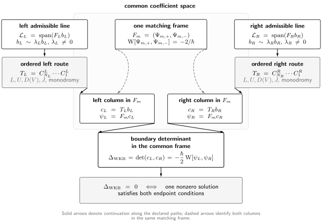
Boundary-to-frame assembly. Each endpoint chooses a projective line; the ordered products $T_L$ and $T_R$ transport those lines through local shears, diagonal Voros transport, sheet exchange, and formal monodromy. Quantization is the vanishing of their wedge in one common frame.

Path order becomes reverse matrix order

Suppose a route encounters $N$ frame changes and Page 4’s source-facing relations are

$$F_{j-1}^{\to j}=F_jC_j, \qquad j=1,\ldots,N.$$

If $c_0$ is the initial coefficient column, then

$$c_j=C_jc_{j-1}.$$

Consequently,

$$T=C_NC_{N-1}\cdots C_1.$$

The first encountered factor acts first on the column and therefore sits furthest to the right in the final product. Reversing this order is one of the most common sources of an apparently plausible but wrong spectral equation.

This $T$ is a source-to-match coefficient transport. If one instead uses Chapter 2’s endpoint relation $F_R=F_LC_{LR}$, then Page 4’s source-facing local relations must be inverted when inserted into $C_{LR}$. Mixing these two matrix directions silently reverses the local shears.

What can appear in the route product

The elementary factors have distinct origins:

$$\begin{aligned} L(s) &= \begin{pmatrix} 1&0\\s&1 \end{pmatrix}, \\ U(s) &= \begin{pmatrix} 1&s\\0&1 \end{pmatrix}, \\ D(V) &= \begin{pmatrix} d_V&0\\0&d_V^{-1} \end{pmatrix}, \\ d_V &:=\ee^{V/2}, \\ J &= \begin{pmatrix} 0&1\\1&0 \end{pmatrix}. \end{aligned}$$

• A simple-zero edge supplies $L(\pm\ii)$ or $U(\pm\ii)$ after the crossing orientation and source-facing convention are fixed.
• A simple-pole edge replaces the Airy multiplier by its exponent-dependent Koike multiplier under the restricted theorem’s hypotheses.
• $D(V)$ changes a normalization endpoint; $V$ is a regularized and directionally summed open or closed Voros exponent.
• $J$ exchanges sheets and branch labels. It is not a Stokes crossing.
• Formal monodromy and singular-endpoint matrices must be inserted when a route winds around a pole or changes an asymptotic sector at infinity.

The entries of $T_L$ and $T_R$ are therefore functions of summed Voros symbols, not merely products of the constants $\pm\ii$.

The exact-WKB passport turns the determinant into a theorem

The algebra above is unconditional once exact frames and exact connection matrices have been supplied. Exact WKB supplies them only after the following hypotheses have been checked on the routes actually used.

1. Normal form and parameter domain. The dependent-variable gauge, contour, open set in $E$, and sector in nonzero $\hbar$ are fixed. Turning points do not coalesce there unless a uniform local model is included.
2. Borel direction. The oriented ray $L_\theta$ and, when singular, its above/below lateral prescription are fixed using the convention of Page 1.
3. Graph chamber. The phased quadratic differential and its Stokes graph are known throughout the continuation. A saddle-free theorem, a lateral resolution, or a stated wall-crossing theorem covers every segment.
4. Cover data. The square-root sheet, branch cuts, lifted paths, closed cycles, and their orientations are fixed.
5. Critical-point hypotheses. Every local shear is justified by the appropriate simple-zero, simple-pole, higher-turning-point, or uniform connection theorem.
6. Endpoint regularization. Turning-point half-contours and pole subtractions are specified. No singular endpoint is treated as an ordinary value-one base point.
7. Summability and uniformity. The WKB series and every quantum part of a Voros exponent used in the product are Borel summable in the chosen direction, uniformly enough for continuation and differentiation.
8. Boundary identification. The summed WKB line is proved to equal the desired regular, recessive, incoming, or outgoing analytic line at each endpoint.
9. Analytic continuation. The finite product follows the declared contour without crossing an unrecorded singularity or changing the spectral sheet.

Under these conditions, the summed WKB frame solves the original ODE, the local and transport matrices are identities between its exact solutions, and $\Delta_{\mathrm{WKB}}$ equals an exact boundary Wronskian up to a nowhere-vanishing analytic factor. Its zeros, with multiplicity, are then exact in the stated parameter domain.

As $E$ varies, the turning points and cycles move. The parameter domain must therefore support a consistent Gauss–Manin transport and avoid discriminants, thresholds, and graph walls not covered by the declared continuation theorem. One printed formula need not extend through all of them.

Exact does not mean symbolically closed

An exact quantization condition may contain Borel sums that must be evaluated numerically. Conversely, a closed elementary expression obtained by truncating a divergent series is not exact. Exactness describes the analytic identity being evaluated; numerical error is a separate layer.

One finite cycle gives a Bohr–Sommerfeld form only after factorization

Consider a real analytic confining potential with two simple real turning points $x_-(E)<x_+(E)$ and

$$p(x,E):=\sqrt{E-V(x)}$$

between them; choose the positive square root. Define the half-action and positive classical action by

$$\begin{aligned} I_0(E) &:=\int_{x_-}^{x_+}p(x,E)\,\dd x, \\ J_0(E)&:=2I_0(E). \end{aligned}$$

Orient the finite WKB cycle $\gamma$ so that

$$\Pi_{\gamma,0}=\ii J_0.$$

Using Page 5’s separation of the classical transmonomial from the quantum power series, first define the chamber-correct quantum correction and resummed period by

$$\begin{aligned} V_{\gamma,\theta}^{\mathrm q} &:=\mathcal S_\theta\widehat V_\gamma^{\mathrm q}, \\ \Pi_{\gamma,\theta}^{\mathrm{sum}} &:=Z_\gamma+\hbar V_{\gamma,\theta}^{\mathrm q}, \\ \mathcal J_\theta &:=-\ii\Pi_{\gamma,\theta}^{\mathrm{sum}}. \end{aligned}$$

At a singular Borel direction, replace $\mathcal S_\theta$ by the declared lateral sum throughout.

Suppose—not merely guess—that the boundary determinant has the factorization

$$\Delta_{\mathrm{WKB}}(E,\hbar) = g(E,\hbar) \left( 1+\mathcal V_{\gamma,\theta} \right),$$

where $g$ is analytic and nowhere zero on the spectral domain. Since

$$\mathcal V_{\gamma,\theta} = \exp\!\left( \frac{\ii\mathcal J_\theta}{\hbar} \right),$$

the boundary condition becomes

$$\mathcal J_\theta(E,\hbar) = 2\pi\hbar \left( n+\frac12 \right), \qquad n\in\mathbb Z,$$

after a continuous logarithm branch has been chosen. The allowed range of $n$ still comes from the spectral domain and boundary problem.

Two Airy shears produce the factor

The simplest two-turning-point topology makes the assumed factorization visible. Choose endpoint frames whose first columns are the left- and right-recessive solutions. Convert Page 4’s source-facing formulae to the endpoint convention $F_R=F_LC_{\mathrm{well}}$, and include the sheet relabeling that puts both Airy crossings into the same lower-triangular form. The audited connection word is then, up to zero-free endpoint normalizations,

$$\begin{aligned} C_{\mathrm{well}} &= L(-\ii)D_vL(-\ii), \\ D_v &= \begin{pmatrix} v^{1/2}&0\\ 0&v^{-1/2} \end{pmatrix}, \\ v &= \mathcal V_{\gamma,\theta}. \end{aligned}$$

The boundary function is the lower-left entry:

$$\begin{aligned} (C_{\mathrm{well}})_{21} &= -\ii \left( v^{1/2}+v^{-1/2} \right) \\ &= -\ii v^{-1/2}(1+v). \end{aligned}$$

The square-root branch affects the nonzero prefactor but not the zero condition. Other frame directions may transpose, conjugate, or invert this word; the invariant calculation is always the wedge of the two admissible lines.

Expanding only formally gives

$$\begin{aligned} \mathcal J_\theta(E,\hbar) \sim{}& J_0(E) + \hbar^2J_2(E) \\ &+ \hbar^4J_4(E) +\cdots. \end{aligned}$$

Keeping just $J_0$ yields the familiar leading rule

$$J_0(E) = 2\pi\hbar \left( n+\frac12 \right).$$

The half-integer shift comes from the two turning-point connection matrices, equivalently from the minus sign in $\mathcal V_\gamma=-1$. It should not be inserted a second time into the definition of the closed quantum period.

The one-cycle formula is not universal

The factorization can fail or acquire more terms when

• additional real wells contribute independent admissible routes;
• complex turning points create active cycles in the chosen direction;
• a barrier or double turning point requires a uniform Weber-type local model;
• a pole changes the local multiplier;
• the boundary conditions are periodic, outgoing, or coupled rather than two-ended recessive;
• a graph wall changes the coordinate chart and the boundary vectors have not been transformed with it.

Page 7 will treat the first nonperturbative corrections and their transseries interpretation. Page 8 will remove the assumption that the important turning points lie on the real axis.

Weber proves the determinant and the cycle equation coincide

Take the real-line oscillator already calibrated in Chapter 8,

$$\begin{gathered} \left[ -\hbar^2\partial_z^2+z^2 \right]\psi = a^2\psi, \\ \hbar>0, \qquad a^2>0. \end{gathered}$$

Set

$$X=\sqrt{\frac2\hbar}\,z, \qquad \nu=\frac{a^2}{2\hbar}-\frac12.$$

Then

$$\frac{\dd^2\psi}{\dd X^2} + \left( \nu+\frac12-\frac{X^2}{4} \right)\psi =0.$$

For real $X$, the right- and left-recessive solutions may be chosen as

$$\psi_R(z)=D_\nu(X), \qquad \psi_L(z)=D_\nu(-X).$$

The parabolic-cylinder Wronskian is

$$\Wr_X[D_\nu(X),D_\nu(-X)] = \frac{\sqrt{2\pi}}{\Gamma(-\nu)}.$$

Reversing the ordered pair and using $\dd X/\dd z=\sqrt{2/\hbar}$ gives

$$\Wr_z[\psi_L,\psi_R] = -\frac{2\sqrt{\pi/\hbar}}{\Gamma(-\nu)}.$$

Normalize away the harmless constant:

$$\Delta_{\mathrm W}(\nu) := -\sqrt{\frac{\hbar}{4\pi}} \Wr_z[\psi_L,\psi_R] = \frac1{\Gamma(-\nu)}.$$

Because the reciprocal gamma function is entire, the boundary determinant vanishes exactly at

$$\nu=n, \qquad n=0,1,2,\ldots.$$

Therefore

$$a_n^2 = (2n+1)\hbar.$$

No semiclassical truncation has entered this calculation. The two-end decay condition and the exact connection coefficient produced the spectrum.

The same zeros appear in one Voros chart

For the cut cycle $\delta$ oriented as in Chapter 8,

$$\Pi_\delta = \ii\pi a^2,$$

and every higher closed Weber period vanishes. Hence

$$\begin{aligned} \mathcal V_\delta &= \exp\!\left( \frac{\ii\pi a^2}{\hbar} \right) \\ &= -\ee^{2\pi\ii\nu}. \end{aligned}$$

Euler’s reflection formula gives the exact factorization

$$\begin{aligned} \Delta_{\mathrm W}(\nu) ={}& \frac{ \Gamma(\nu+1)\ee^{-\pi\ii\nu} }{2\pi\ii} \\ &\times \left( 1+\mathcal V_\delta \right). \end{aligned}$$

On the physical domain $a^2>0$, equivalently $\nu>-1/2$, the prefactor is analytic and nowhere zero. Thus

$$\Delta_{\mathrm W}=0 \quad\Longleftrightarrow\quad 1+\mathcal V_\delta=0$$

there. This is a proof that the simple cycle equation is an exact quantization condition for this boundary problem.

Outside that domain, $1+\mathcal V_\delta$ also vanishes at negative integers. Those apparent roots are canceled by poles of $\Gamma(\nu+1)$ in the full boundary determinant. The example makes Page 5’s warning concrete: a Voros factor by itself does not know the admissible spectral domain or endpoint normalization.

The cycle here is Chapter 8’s $\delta_{\mathrm{cut}}$. It is not Page 5’s oppositely oriented active wall class at $\theta=\pi/2$.

Every Weber eigenvalue is simple

Near $\nu=n\geq0$,

$$\begin{aligned} \Delta_{\mathrm W}(\nu) ={}& (-1)^{n+1}n! (\nu-n) \\ &+ O\!\left((\nu-n)^2\right). \end{aligned}$$

Therefore

$$\left. \frac{\partial\Delta_{\mathrm W}}{\partial a^2} \right|_{a^2=(2n+1)\hbar} = \frac{(-1)^{n+1}n!}{2\hbar} \neq0.$$

The determinant detects not only the root locations but their simplicity. Multiplying it by a zero-free analytic factor changes the derivative’s value, but not whether the derivative vanishes at a root.

The same equation has two different half-line spectra

On $z\geq0$, the right-recessive solution is still $D_\nu(X)$. Dirichlet and Neumann conditions at the regular endpoint use the exact values below, where the prime differentiates with respect to $X$:

$$\begin{aligned} D_\nu(0) &= \frac{ 2^{\nu/2}\sqrt\pi }{ \Gamma\!\left((1-\nu)/2\right) }, \\ D_\nu'(0) &= -\frac{ 2^{(\nu+1)/2}\sqrt\pi }{ \Gamma(-\nu/2) }. \end{aligned}$$

After removing nonzero factors, the two boundary functions are

$$\begin{aligned} \Delta_D(\nu) &= \frac1{ \Gamma\!\left((1-\nu)/2\right) }, \\ \Delta_N(\nu) &= \frac1{ \Gamma(-\nu/2) }. \end{aligned}$$

Their roots give

$$\begin{array}{c|c|c} \text{condition at }0 &\nu &a^2 \\ \hline \text{Dirichlet} &2m+1 &(4m+3)\hbar \\ \text{Neumann} &2m &(4m+1)\hbar \end{array}$$

for $m\geq0$. The two sequences are the odd and even full-line states. The differential equation and recessive condition at $+\infty$ are the same; changing the condition at $0$ changes the spectrum.

Other boundary problems change the scalar equation

The transported-line construction is not restricted to bound states.

A connection entry for separated endpoint lines

Suppose local ordered frames have their first columns equal to the selected endpoint solutions and

$$F_R=F_LC_{LR}.$$

Then the right selected solution is

$$\psi_R = (C_{LR})_{11}\psi_L + (C_{LR})_{21}\widetilde\psi_L.$$

The spectral condition is

$$(C_{LR})_{21}=0.$$

Reordering either basis changes the vanishing entry. The invariant statement is that the selected lines intersect, or equivalently that their Wronskian vanishes.

Bloch conditions use monodromy, not two recessive lines

Let $M(E,\hbar)$ be the exact one-period monodromy in an ordered frame and let $\mu_B$ be the declared Bloch multiplier. A Bloch solution exists when

$$\Delta_{\mu_B}(E,\hbar) := \det\!\left( M(E,\hbar)-\mu_BI \right) =0.$$

If $M\in SL(2,\mathbb C)$, then

$$\Delta_{\mu_B} = \mu_B^2 - \mu_B\operatorname{tr}M +1.$$

For $\mu_B=\ee^{\ii kL}$ this becomes

$$\operatorname{tr}M = 2\cos(kL).$$

The exact-WKB task is now to compute the monodromy product, including formal monodromy and every Stokes/Voros factor. At periodic and antiperiodic band edges, $\mu_B=+1$ and $-1$ respectively.

The equality $\operatorname{tr}M=\pm2$ guarantees a periodic or antiperiodic eigenline. It does not by itself imply that $M=\pm I$, that two independent Bloch solutions exist, or that the band edge is simple.

Resonances use outgoing lines on a continued sheet

For a resonance or quasinormal problem, choose the outgoing or ingoing canonical line at each contour end and continue both on the declared spectral sheet. Their Wronskian again supplies a scalar condition. Its zeros are generally complex, and the identification of those zeros with poles of a continued resolvent is an additional theorem from spectral theory.

Nothing in the determinant algebra forces self-adjointness, reality, or stability. Those properties come from the operator domain, symmetries, and sheet structure.

Chamber changes act on the whole boundary problem

Let two WKB frames on opposite lateral determinations satisfy

$$F_m^+=F_m^-G,$$

where $G$ is the relevant Stokes or wall-crossing matrix. A fixed exact solution has coefficients related by

$$c^+=G^{-1}c^-.$$

Therefore

$$\det(c_L^+,c_R^+) = \det(G^{-1}) \det(c_L^-,c_R^-).$$

For the unit-Wronskian shears of Pages 4–5, $\det G=1$, so the determinant is unchanged. More general analytic frame renormalizations multiply it by a nowhere-zero factor. In either case, the consistently continued zero divisor is invariant.

By contrast, applying the DDP substitution to a Voros symbol while leaving the endpoint vectors or the rest of the route product in the old chamber mixes two coordinate charts. The resulting scalar need not represent the same boundary problem and may acquire spurious zeros.

On an actually singular Borel ray, the two lateral determinants are distinct prescribed objects until a theorem identifies their physical completion. The covariance calculation does not, by itself, prove median summability or ambiguity cancellation; Page 7 supplies that extra layer.

A useful wall-crossing test

Compute the boundary determinant independently on the two sides of a wall. After transporting every cycle, path, frame, and endpoint line, their ratio should be analytic and nowhere zero on the overlap. Equality is expected only when the two normalizations were chosen identically.

Multiplicity is a zero-divisor statement

Assume $\Delta(E)$ is analytic near an isolated root $E_*$ and is not identically zero. The root multiplicity is

$$m = \operatorname{ord}_{E_*}\Delta.$$

Equivalently, for a small positively oriented circle $C_*$ containing no other zero,

$$m = \frac{1}{2\pi\ii} \oint_{C_*} \frac{\Delta'(E)}{\Delta(E)} \,\dd E.$$

This contour count is invariant under $\Delta\mapsto g\Delta$ with $g$ analytic and nowhere zero. A simple root has $\Delta'(E_*)\neq0$; a multiple root requires further derivatives.

For a holomorphic Fredholm pencil of index zero, a suitably normalized characteristic function can encode algebraic multiplicity. Without those operator hypotheses, the order of a chosen scalar boundary function should not automatically be called the algebraic multiplicity of an operator eigenvalue.

Likewise, a boundary Wronskian is not automatically a Fredholm determinant, a zeta-regularized determinant, or a canonical product. Chapter 2 states the additional hypotheses and comparison theorems for those objects.

For the real Schrödinger problem, differentiation gives the useful local identity

$$\frac{\dd}{\dd x} \Wr[\psi,\partial_E\psi] = -\frac{\psi^2}{\hbar^2}.$$

If the endpoint conditions and normalizations are $E$-independent in the required Lagrange-bracket sense, and $\psi_R=\kappa\psi_L=\kappa\psi$ at an eigenvalue, integration yields

$$\Delta'(E_n) = \frac{\kappa}{\hbar^2} \int_{x_L}^{x_R}\psi(x)^2\,\dd x$$

for the corresponding raw boundary Wronskian. There is no complex conjugation in this analytic identity. In a real self-adjoint problem the integral proves simplicity; in a nonselfadjoint problem the proper derivative test generally involves an adjoint mode.

Numerically, three checks are especially valuable:

1. evaluate the Wronskian at several regular matching points;
2. compare two independent normalizations and verify that their ratio is nonzero near the root;
3. use a contour count or derivative test rather than relying only on a small plotted value of $|\Delta|$.

A reproducible boundary-to-spectrum workflow

For a concrete exact-WKB spectral calculation, proceed in this order.

1. State the differential expression, contour, function space or radiation problem, and spectral parameter domain.
2. Fix the time convention and spectral sheet when outgoing or ingoing conditions are used.
3. Put the equation in Schrödinger normal form and retain the inverse gauge map for the original boundary data.
4. Fix $\arg\hbar$, the Borel ray $L_\theta$, the graph chamber, and any lateral prescription.
5. Draw the phased Stokes graph and choose the cover sheet, cuts, cycles, lifted paths, and orientations.
6. Identify the exact analytic line selected at each endpoint. Do not use a formal decay mnemonic at a threshold or singular endpoint.
7. Choose local WKB frames and represent the endpoint lines by coefficient columns $b_L$ and $b_R$.
8. Choose one matching frame and record every source-facing relation $F_{j-1}^{\to j}=F_jC_j$.
9. Assemble $T_L$ and $T_R$ in path order, including local shears, diagonal Voros transports, sheet exchanges, and formal monodromy.
10. Form $\Delta_{\mathrm{WKB}}=\det(T_Lb_L,T_Rb_R)$ and verify its Wronskian normalization.
11. Prove that the summed frames and matrices satisfy the analytic passport; label the result conditional if any theorem hypothesis remains open.
12. Solve the scalar equation with controlled summation, truncation, and root-finding error, then check it against an independent method.

This sequence separates a geometry error, a matrix-order error, a boundary error, and a numerical error before they can compensate accidentally.

Computational audit

The companion script exact-quantization-check.py checks the finite-dimensional identities and the Weber calibration. It verifies

• the determinant–Wronskian relation for a general coefficient pair;
• source-facing route order and determinant-one covariance;
• the two-shear factor $1+\mathcal V$;
• the parabolic-cylinder Wronskian at several regular points;
• the reciprocal-gamma/Voros factorization at real and complex $\nu$;
• the first seven Weber roots, their derivatives, and the cancellation of negative-integer cycle roots;
• the half-line Dirichlet/Neumann parity split and Hermite states;
• the $SL(2)$ Bloch characteristic polynomial.

These tests do not prove Borel summability, endpoint admissibility, graph completeness, or the applicability of a local connection theorem to a new potential.

Common pitfalls

Quantizing the printed ODE. An ODE has a two-dimensional solution space, not a preferred spectrum. State the operator domain or radiation problem before solving a scalar equation.

Setting one Voros factor to $-1$ by pattern recognition. The equation $1+\mathcal V_\gamma=0$ is spectral only after the transported boundary determinant is shown to have that factor with a zero-free remainder. Weber shows both why the rule works and how it can acquire spurious roots outside the declared domain.

Multiplying matrices in drawing order. With row frames and coefficient columns, the first encountered source-facing matrix is the rightmost factor in the final product. Derive the update $c_j=C_jc_{j-1}$ before coding.

Using a formal period as an analytic number. A divergent all-orders period must be summed in a specified direction and chamber. Optimal truncation or Borel–Padé is a numerical approximation, not the definition of the exact symbol.

Changing the frame but not the boundary vector. Coefficients transform contragrediently. A Stokes or wall-crossing transformation applied to only one part of the determinant mixes conventions and can move its zeros.

Reading multiplicity from a normalization-dependent slope. A zero-free factor changes $\Delta'(E_*)$. It preserves the order of the zero, which is the invariant datum.

Exercises

1. Prove the determinant–Wronskian identity

Let $F=(f_+,f_-)$ and $u=Fc$, $v=Fd$. Show that

$$\Wr[u,v] = \det(c,d)\Wr[f_+,f_-].$$

Specialize to the unit WKB normalization.

Solution

Write $u=c_+f_++c_-f_-$ and $v=d_+f_++d_-f_-$. Bilinearity and antisymmetry leave only the two cross terms:

$$\begin{aligned} \Wr[u,v] &= c_+d_-\Wr[f_+,f_-] \\ &\quad+ c_-d_+\Wr[f_-,f_+] \\ &= (c_+d_--c_-d_+) \Wr[f_+,f_-]. \end{aligned}$$

The coefficient in parentheses is $\det(c,d)$. For $\Wr[f_+,f_-]=-2/\hbar$,

$$\det(c,d) = -\frac\hbar2\Wr[u,v].$$

2. Convert a Robin condition into a line

For $F=(f_+,f_-)$ at $z=a$, impose

$$\alpha\psi(a)+\beta\hbar\psi'(a)=0.$$

Find a coefficient column spanning the admissible line.

Solution

Define

$$\begin{aligned} \ell_+ &= \alpha f_+(a)+\beta\hbar f_+'(a), \\ \ell_- &= \alpha f_-(a)+\beta\hbar f_-'(a). \end{aligned}$$

The boundary condition is $\ell_+c_++\ell_-c_-=0$, so one spanning column is

$$b= \begin{pmatrix} -\ell_-\\\ell_+ \end{pmatrix}.$$

Indeed $\ell^{\mathsf T}b=0$. Any nonzero scalar multiple represents the same projective line.

3. Derive the route-product order

Suppose

$$\begin{aligned} F_0^{\to1} &=F_1C_1, \\ F_1^{\to2} &=F_2C_2, \\ F_2^{\to3} &=F_3C_3. \end{aligned}$$

If $\psi=F_0c_0$, find its coefficient column in $F_3$.

Solution

At the first step,

$$\psi=F_1C_1c_0,$$

so $c_1=C_1c_0$. Repeating the argument gives

$$c_2=C_2C_1c_0, \qquad c_3=C_3C_2C_1c_0.$$

Thus the first encountered matrix is the rightmost factor.

4. Check matching-frame covariance

Let $F_m^+=F_m^-G$ with $G$ invertible. Derive the transformation of the two coefficient columns and their determinant.

Solution

For a fixed solution,

$$F_m^-c^- = F_m^+c^+ = F_m^-Gc^+.$$

Hence $c^+=G^{-1}c^-$. Applying this to both endpoint lines gives

$$\det(c_L^+,c_R^+) = \det(G^{-1}) \det(c_L^-,c_R^-).$$

If $G\in SL(2)$, the determinant is unchanged. For a general analytic frame change it is multiplied by a nowhere-zero factor.

5. Recover the Weber boundary determinant

Use

$$D_\nu(X)=U\!\left(-\nu-\frac12,X\right)$$

and

$$\Wr_X[U(A,X),U(A,-X)] = \frac{\sqrt{2\pi}}{\Gamma(A+1/2)}$$

to compute $\Wr_z[D_\nu(-X),D_\nu(X)]$ for $X=\sqrt{2/\hbar}\,z$.

Solution

Set $A=-\nu-1/2$. Then

$$\Wr_X[D_\nu(X),D_\nu(-X)] = \frac{\sqrt{2\pi}}{\Gamma(-\nu)}.$$

Reversing the pair changes the sign, and changing variables contributes $\dd X/\dd z=\sqrt{2/\hbar}$. Therefore

$$\Wr_z[D_\nu(-X),D_\nu(X)] = -\frac{2\sqrt{\pi/\hbar}}{\Gamma(-\nu)}.$$

Multiplication by $-\sqrt{\hbar/(4\pi)}$ gives $\Delta_{\mathrm W}=1/\Gamma(-\nu)$.

6. Factor the Weber determinant through its cycle symbol

Starting from Euler’s reflection formula and $\mathcal V_\delta=-\ee^{2\pi\ii\nu}$, prove

$$\frac1{\Gamma(-\nu)} = \frac{ \Gamma(\nu+1)\ee^{-\pi\ii\nu} }{2\pi\ii} \left( 1+\mathcal V_\delta \right).$$

Why is the equivalence of zero sets restricted to a domain?

Solution

Reflection gives

$$\frac1{\Gamma(-\nu)} = -\frac{\Gamma(\nu+1)\sin(\pi\nu)}{\pi}.$$

Also,

$$1+\mathcal V_\delta = 1-\ee^{2\pi\ii\nu} = -2\ii\ee^{\pi\ii\nu} \sin(\pi\nu).$$

Combining the two identities proves the formula. The prefactor is analytic and nonzero on $\nu>-1/2$, but has poles at negative integers. Globally those poles cancel the additional zeros of $1+\mathcal V_\delta$, so the two factors do not have the same zero divisor on the whole plane.

7. Verify Weber simplicity

Show that

$$\left. \frac{\dd}{\dd\nu} \frac1{\Gamma(-\nu)} \right|_{\nu=n} = (-1)^{n+1}n!$$

for $n\geq0$.

Solution

Near $z=-n$, gamma has the simple pole

$$\Gamma(z) = \frac{(-1)^n}{n!(z+n)} +O(1).$$

Put $z=-\nu$ and $\nu=n+\varepsilon$. Then $z+n=-\varepsilon$, so

$$\frac1{\Gamma(-\nu)} = (-1)^{n+1}n!\,\varepsilon +O(\varepsilon^2).$$

The stated derivative follows and is nonzero.

8. Derive the Bloch trace condition

Let $M\in SL(2,\mathbb C)$. Show that

$$\det(M-\mu I) = \mu^2-\mu\operatorname{tr}M+1.$$

Set $\mu=\ee^{\ii kL}$.

Solution

For a $2\times2$ matrix,

$$\det(M-\mu I) = \mu^2-\mu\operatorname{tr}M+\det M.$$

Since $\det M=1$, the displayed polynomial follows. Dividing its zero condition by $\mu\neq0$ gives

$$\operatorname{tr}M = \mu+\mu^{-1} = 2\cos(kL).$$

9. Preview the first instanton displacement

Suppose a chamber-labelled boundary function has the formal action-graded form

$$\begin{aligned} \mathcal Q(E,\hbar) ={}& \mathcal Q_0(E,\hbar) \\ &+ \sigma\ee^{-A/\hbar} \mathcal Q_1(E,\hbar) +\cdots, \end{aligned}$$

and $\mathcal Q_0(E_0,\hbar)=0$ with $\partial_E\mathcal Q_0(E_0,\hbar)\neq0$. Find the first displacement of the root.

Solution

Put $E=E_0+\delta E$ and expand to first order in the instanton monomial. Then

$$\begin{aligned} 0 ={}& \partial_E\mathcal Q_0(E_0,\hbar) \,\delta E \\ &+ \sigma\ee^{-A/\hbar} \mathcal Q_1(E_0,\hbar) +\cdots. \end{aligned}$$

Therefore

$$\delta E = -\sigma\ee^{-A/\hbar} \frac{ \mathcal Q_1(E_0,\hbar) }{ \partial_E\mathcal Q_0(E_0,\hbar) } +\cdots.$$

This is only the first formal displacement. The lateral dependence of $\sigma$, higher sectors, logarithms, and ambiguity cancellation are the subject of Page 7.

From quantization to transseries

This page treated the boundary determinant as the primary object and showed when it reduces to a one-cycle equation. In a multiwell problem or near a graph wall, the determinant contains exponentially small symbols from additional cycles. Solving it then shifts a perturbative root by an instanton series; lateral ambiguities of the perturbative sector must cancel those of the nonperturbative sectors.

Page 7 derives that mechanism from the determinant rather than appending an instanton term by hand.

References

• Voros, A., “The Return of the Quartic Oscillator: The Complex WKB Method”, Annales de l’Institut Henri Poincaré A 39 (1983), 211–338. Develops exact resummation, complex connection data, and spectral functions for one-dimensional Schrödinger problems.
• Delabaere, E., Dillinger, H., and Pham, F., “Exact Semiclassical Expansions for One-Dimensional Quantum Oscillators”, Journal of Mathematical Physics 38 (1997), 6126–6184. Gives rigorous exact-WKB quantization rules for simple and double oscillators and the multi-instanton extension used on the next page.
• Delabaere, E., and Pham, F., “Resurgent Methods in Semi-Classical Asymptotics”, Annales de l’Institut Henri Poincaré A 71 (1999), 1–94. Systematic treatment of resurgent WKB solutions, connection problems, and spectral applications.
• Kawai, T., and Takei, Y., Algebraic Analysis of Singular Perturbation Theory, Translations of Mathematical Monographs 227, American Mathematical Society, 2005, especially Chapters 2–3. Standard exact-WKB connection and global monodromy framework.
• Nikolaev, N., “Existence and Uniqueness of Exact WKB Solutions for Second-Order Singularly Perturbed Linear ODEs”, Communications in Mathematical Physics 400 (2023), 463–517. Modern existence, uniqueness, basis, and Borel-summability theorems for exact WKB solutions on stated trajectory domains.
• Iwaki, K., “Les Houches Lectures on Exact WKB Analysis and Painlevé Equations”, lecture notes, revised 2026, especially §1.4. Derives global Stokes matrices as products of local connection factors and Borel-summed Voros periods, including the Weber calibration.
• NIST Digital Library of Mathematical Functions, §12.2(iii), Wronskians and §12.9(i), large-variable asymptotics. Authoritative parabolic-cylinder identities used for the exact Weber boundary determinant and recessive sectors.
• Teschl, G., Mathematical Methods in Quantum Mechanics, second edition, American Mathematical Society, 2014. Background on one-dimensional Schrödinger operators, boundary conditions, and spectral multiplicity; exact-WKB input is separate.