The Nekrasov–Shatashvili Limit and Twisted Superpotential

Page 3 constructed a finite two-parameter object, $Z_{\mathrm{Nek}}(\epsilon_1,\epsilon_2)$. The Nekrasov–Shatashvili limit does not evaluate that object at $\epsilon_2=0$. It extracts the coefficient of its divergent connected free energy while the other rotation remains finite:

$$\mathcal W_{\mathrm{NS}}^{\mathrm{loc}} := \lim_{\epsilon_2\to0} \epsilon_2 \log Z_{\mathrm{Nek}} \left( \epsilon_1=\hbar, \epsilon_2 \right).$$

After a Barnes subtraction, a logarithm sheet, and a parameter chamber have been fixed, this limit is a two-dimensional effective twisted superpotential. It is neither the four-dimensional prepotential nor the partition function itself. It also does not, by itself, specify a quantum differential operator, a wavefunction, a WKB cycle, or a complete exact spectrum. Those distinctions are the organizing principle of this page.

Page question

Which coefficient of the full Nekrasov function survives the anisotropic Omega-background limit, how can it be computed and checked, and what extra choices are required before its critical equations become a physical spectral problem?

Status ledger

Statement used on this page	Status
$\epsilon_2\to0$ with $\epsilon_1$ fixed	Definition of this NS limit; $\hbar:=\epsilon_1$ is only a page-local abbreviation until Pages 5–6 supply an ODE dictionary
$\mathcal W_{\mathrm{NS}}^{\mathrm{loc}}=\lim\epsilon_2\log Z_{\mathrm{Nek}}$	Definition whenever the connected free energy has the stated leading simple pole; the standard NS asymptotic is conditional on the declared chamber and contour, and the pure-$SU(2)$ instanton sector is checked here through $\mathfrak q^2$
$Z_{\mathrm{Nek}}\vert_{\epsilon_2=0}$ is the NS object	False; $Z_{\mathrm{Nek}}$ is generally exponentially singular
The logarithm can be taken after the limit	False; connected and disconnected poles must cancel first
The NS limit leaves a two-dimensional twisted F-term	Exact low-energy interpretation in the preserved supersymmetric sector
$\mathcal W_{\mathrm{NS}}$ equals the Seiberg–Witten prepotential	False; $\hbar\mathcal W_{\mathrm{NS}}\to\mathscr F_0=-2\pi\ii\mathcal F_{\mathrm{SW}}$ in this book’s convention
$\exp(\partial_{a^i}\mathcal W_{\mathrm{eff}})=1$	Branch-independent vacuum equation when $a^i$ are dynamical two-dimensional Coulomb variables
Every solution of that equation is an exact ODE eigenvalue	False
“All instantons” is an all-orders formal series in $\mathfrak q$	True; it is nonperturbative in the microscopic gauge coupling because $\mathfrak q\sim e^{2\pi\ii\tau}$
“All instantons” is automatically a nonperturbative completion in $\hbar$	False
A pole at $2a=\pm n\hbar$, $n\in\mathbb Z_{>0}$, is automatically a physical level	False; it is first an equivariant resonance of the chosen expansion

Convention ledger

Datum	Convention on this page
Surviving weight	$\epsilon_1=\hbar$ is fixed; it is not yet identified with an ODE Planck constant
Vanishing weight	$\epsilon_2\to0$ in a chosen punctured parameter chamber
Full input	$Z_{\mathrm{Nek}}:=Z_{\mathrm{cl}}Z_{\mathrm{1-loop}}Z_{\mathrm{inst}}$
Local NS object	$\mathcal W_{\mathrm{NS}}^{\mathrm{loc}}:=\lim\epsilon_2\log Z_{\mathrm{Nek}}$
NS free energy	$\mathscr F_{\mathrm{NS}}^{\mathrm{loc}}:=\hbar\mathcal W_{\mathrm{NS}}^{\mathrm{loc}}$
Flat limit	$\mathscr F_{\mathrm{NS}}^{\mathrm{loc}}\to\mathscr F_0=-2\pi\ii\mathcal F_{\mathrm{SW}}$
Instanton branch	Formal logarithm at $Z_{\mathrm{inst}}=1+O(\mathfrak q)$
Perturbative branch	Continued from one declared Coulomb/mass chamber with the Page 3 Barnes subtraction
Mass held fixed	The Page 3 equivariant label $\boldsymbol\mu$; centered masses retain their finite $\hbar/2$ shift
Physical superpotential	$\mathcal W_{\mathrm{eff}}=\mathcal W_{\mathrm{NS}}^{\mathrm{loc}}+\mathcal W^\infty$ when boundary data require $\mathcal W^\infty$
Series status	Formal in $\mathfrak q$ unless a convergence domain, contour, or resummation is stated
Excluded limits	The self-dual slice $\epsilon_1+\epsilon_2=0$ is not NS; the exchanged anisotropic limit $\epsilon_1\to0$ at fixed $\epsilon_2$ is not taken here, although the later sequential flat check sends $\hbar\to0$ after the NS limit

The limit is a connected simple-pole coefficient

Fix a punctured neighborhood of $\epsilon_2=0$, set $\epsilon_1=\hbar\ne0$, and continue all parameters without crossing a chosen pole or logarithm cut. After the same local subtractions used on Page 3, the relevant asymptotic form is

$$\log Z_{\mathrm{Nek}} = \frac{ \mathcal W_{\mathrm{NS}}^{\mathrm{loc}} }{\epsilon_2} + R_{\mathrm{NS}}(\epsilon_2), \qquad R_{\mathrm{NS}}(\epsilon_2) =o(\epsilon_2^{-1}).$$

Thus $\mathcal W_{\mathrm{NS}}^{\mathrm{loc}}$ is equivalently the $\epsilon_2^{-1}$ coefficient of $\log Z_{\mathrm{Nek}}$. The remainder may contain constants or saddle-fluctuation terms such as $\log\epsilon_2$; none changes the limit after multiplication by $\epsilon_2$. The superscript “loc” reminds us that this is the universal holomorphic block on $\mathbb C^2$ with Coulomb data fixed at infinity. Later boundary terms can change the physical effective superpotential.

Exponentiating the asymptotic series gives

$$Z_{\mathrm{Nek}} = \exp\!\left[ \frac{ \mathcal W_{\mathrm{NS}}^{\mathrm{loc}} }{\epsilon_2} \right] \exp\!\left[ R_{\mathrm{NS}}(\epsilon_2) \right].$$

Unless the twisted superpotential vanishes, direct substitution $\epsilon_2=0$ therefore meets an essential exponential singularity. Multiplication by $\epsilon_2$ does not repair $Z$; it repairs its logarithm. This is why the order

$$Z \longrightarrow \log Z \longrightarrow \epsilon_2\log Z \longrightarrow \epsilon_2\to0$$

is part of the definition rather than a computational preference.

Why a two-dimensional superpotential survives

Write the equivariant spacetime as

$$\mathbb R^4 \simeq \mathbb R^2_{\epsilon_1} \times \mathbb R^2_{\epsilon_2}.$$

At generic nonzero $(\epsilon_1,\epsilon_2)$, both planes are rotated. When $\epsilon_2\to0$, translations return along the second plane while the first remains Omega-deformed with weight $\hbar$. The surviving sector has two-dimensional $\mathcal N=(2,2)$ supersymmetry, or four supercharges. Its twisted F-terms are encoded by a twisted superpotential.

The factor $1/\epsilon_2$ is the equivariant volume of the plane whose rotation is being removed. This also fixes the units:

$$[\log Z]=0, \qquad [\epsilon_2]=1, \qquad [\mathcal W_{\mathrm{NS}}]=1.$$

A derivative with respect to a Coulomb parameter is consequently dimensionless and may be exponentiated in a vacuum equation. Nothing in this dimensional argument identifies $\hbar$ with the Planck constant of a particular ODE. That identification needs the quantum curve and normalization data of Pages 5–6.

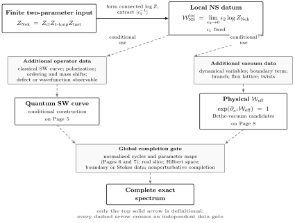
Only the top solid arrow is the NS definition. Every dashed arrow crosses an independent data gate: neither a quantum Seiberg–Witten curve nor Bethe-vacuum candidates follow from $\mathcal W_{\mathrm{NS}}^{\mathrm{loc}}$ alone, and a complete spectrum additionally requires normalized cycles, a real or complex spectral slice, boundary or Stokes data, and a nonperturbative completion.

Classical, one-loop, and instanton sectors remain distinct

Use the full-function convention of Page 3:

$$Z_{\mathrm{Nek}} = Z_{\mathrm{cl}} Z_{\mathrm{1-loop}} Z_{\mathrm{inst}}.$$

Because the logarithm turns products into sums, define in one common scheme

$$\begin{aligned} \mathcal W_{\mathrm{NS}}^{\mathrm{cl}} &:= \lim_{\epsilon_2\to0} \epsilon_2\log Z_{\mathrm{cl}}, \\ \mathcal W_{\mathrm{NS}}^{\mathrm{1-loop}} &:= \lim_{\epsilon_2\to0} \epsilon_2\log Z_{\mathrm{1-loop}}, \\ \mathcal W_{\mathrm{NS}}^{\mathrm{inst}} &:= \lim_{\epsilon_2\to0} \epsilon_2\log Z_{\mathrm{inst}}. \end{aligned}$$

Then

$$\begin{aligned} \mathcal W_{\mathrm{NS}}^{\mathrm{loc}} &= \mathcal W_{\mathrm{NS}}^{\mathrm{pert}} + \mathcal W_{\mathrm{NS}}^{\mathrm{inst}}, \\ \mathcal W_{\mathrm{NS}}^{\mathrm{pert}} &:= \mathcal W_{\mathrm{NS}}^{\mathrm{cl}} + \mathcal W_{\mathrm{NS}}^{\mathrm{1-loop}}. \end{aligned}$$

Calling the positive-instanton term “the NS superpotential” silently drops the classical coupling and the perturbative determinant. That abbreviation is especially dangerous in vacuum equations because all three pieces contribute to Coulomb derivatives.

The classical term

For the conformal classical factor declared on Page 3,

$$Z_{\mathrm{cl}} = \exp\!\left[ - \frac{ \log q_{\mathrm{UV}} }{2\epsilon_1\epsilon_2} (\boldsymbol a,\boldsymbol a) \right],$$

the limit is immediate:

$$\mathcal W_{\mathrm{NS}}^{\mathrm{cl}} = - \frac{ \log q_{\mathrm{UV}} }{2\hbar} (\boldsymbol a,\boldsymbol a).$$

On the traceless pure-$SU(2)$ slice $(a_1,a_2)=(a,-a)$, the same printed expression would be

$$\mathcal W_{\mathrm{NS}}^{\mathrm{cl},SU(2)} = -\frac{a^2}{\hbar} \log q_{\mathrm{UV}}.$$

For an asymptotically free theory, however, the cutoff-dependent classical term and the running one-loop determinant must be combined. The dimensionful instanton fugacity $\mathfrak q=\Lambda^{b_0}$ is not inserted into a conformal logarithm formula as if it were $q_{\mathrm{UV}}$.

The Barnes determinant collapses to a Gamma kernel

Let $\gamma_{\epsilon_1,\epsilon_2}(x)$ be precisely the Barnes double-zeta function fixed on Page 3, with subtraction scale $M$. Define its one-parameter NS reduction by

$$\omega_\hbar(x;M) := \lim_{\epsilon_2\to0} \epsilon_2 \gamma_{\hbar,\epsilon_2}(x).$$

In the initial convergence chamber and then by analytic continuation on a chosen logarithm branch,

$$\begin{aligned} \omega_\hbar(x;M) = -\hbar\Bigg[ &\zeta_H'\!\left( -1,1+\frac{x}{\hbar} \right) \\ &+ \left( 1+\log\frac{M}{\hbar} \right) \zeta_H\!\left( -1,1+\frac{x}{\hbar} \right) \Bigg], \end{aligned}$$

where $\zeta_H$ is the Hurwitz zeta function and the prime differentiates its first argument. More useful in computations is

$$\begin{aligned} \omega_\hbar'(x;M) = {}&- \log\Gamma\!\left( 1+\frac{x}{\hbar} \right) +\frac12\log(2\pi) \\ &+ \left( \frac{x}{\hbar}+\frac12 \right) \log\frac{M}{\hbar}. \end{aligned}$$

This formula makes three subtleties visible. A logarithm branch is required; $\Gamma$ has poles when its argument reaches a nonpositive integer, so $\omega_\hbar'$ has logarithmic branch singularities there; and changing the Barnes subtraction adds a local polynomial. For general matter content, one evaluates $\omega_\hbar$ on the root and weight arguments inherited from the Page 3 factor library, including all $\hbar$-dependent shifts. One should not reconstruct those shifts from memory after the limit.

For example, the local vector contribution of pure $SU(2)$ in that exact library is

$$\begin{aligned} \mathcal W_{\mathrm{NS}}^{\mathrm{vec}} = {}&- \omega_\hbar(2a-\hbar;M) \\ &- \omega_\hbar(2a;M). \end{aligned}$$

Combining it with the running classical term, $q_{\mathrm{UV}}(M)=\Lambda^4/M^4$, gives, up to the declared local counterterm and branch freedom,

$$\begin{aligned} \frac{\partial \mathcal W_{\mathrm{NS}}^{\mathrm{pert}} }{\partial a} = {}&2\log\!\left[ \frac{ \Gamma(2a/\hbar) \Gamma(1+2a/\hbar) }{2\pi} \right] \\ &+ \frac{8a}{\hbar} \log\frac{\hbar}{\Lambda}. \end{aligned}$$

This is a chamber formula, not a globally single-valued function of $a/\hbar$. Stirling expansion gives the expected weak-coupling behavior

$$\hbar \frac{\partial \mathcal W_{\mathrm{NS}}^{\mathrm{pert}} }{\partial a} = 8a\log\frac{a}{\Lambda} + \text{a scheme-dependent linear term} +O(\hbar).$$

The logarithmic part matches the Page 2 dual-period asymptotics after using this chapter’s localization sign. Once $q_{\mathrm{UV}}(M)=\Lambda^4/M^4$ runs consistently, a pure change of $M$ cancels from the $a$-dependent derivative. The linear term can move under an unmatched subtraction-scale or finite-coupling redefinition, a quadratic counterterm, a logarithm sheet, or an integral change of the magnetic cycle.

The mass shift survives the limit

Page 3 distinguished an equivariant mass label $\mu$ from a centered physical mass $\widehat m=\mu-\epsilon_\Sigma/2$. In the NS limit, $\epsilon_\Sigma\to\hbar$, so $\widehat m=\mu-\hbar/2$. Holding $\mu$ fixed and then silently calling it $\widehat m$ changes finite-$\hbar$ formulas and later quantum-curve potentials.

Pure SU(2) through two instantons

The instanton sector provides a sharp audit because it is independent of the perturbative Barnes subtraction once the fugacity, masses, and decoupled Abelian factors have been fixed. Write

$$Z_{\mathrm{inst}} = 1+ \mathfrak q Z_1+ \mathfrak q^2 Z_2+ O(\mathfrak q^3).$$

Its formal logarithm around the empty-partition term is

$$\log Z_{\mathrm{inst}} = \mathfrak q Z_1 + \mathfrak q^2 \left( Z_2-\frac12Z_1^2 \right) + O(\mathfrak q^3).$$

The combinations in parentheses are cumulants: they remove disconnected repetitions of lower-instanton configurations. At order $\mathfrak q^k$, the connected combination can have a simple $1/\epsilon_2$ pole even though the individual $Z_j$ contain powers as high as $1/\epsilon_2^j$. This cancellation is the instanton version of the ordinary statement that $\log Z$ generates connected vacuum diagrams.

Adopt the Page 3 pure-$SU(2)$ data

$$(a_1,a_2)=(a,-a), \qquad \Delta:=2a, \qquad \mathfrak q=\Lambda^4,$$

and abbreviate $\epsilon_2=\varepsilon$ while taking the limit. The exact one-instanton coefficient is

$$Z_1 = -\frac{2}{ \hbar\varepsilon \left[ \Delta^2-(\hbar+\varepsilon)^2 \right] }.$$

Hence

$$\lim_{\varepsilon\to0} \varepsilon Z_1 = -\frac{2}{ \hbar(\Delta^2-\hbar^2) }.$$

At two instantons, Page 3 reduced the five fixed-point contributions to the connected expression

$$\begin{aligned} Z_2-\frac12Z_1^2 ={}&- \frac{ 5\Delta^2+7\hbar^2 +16\hbar\varepsilon+7\varepsilon^2 }{ \hbar\varepsilon \left[ \Delta^2-(\hbar+\varepsilon)^2 \right]^2 } \\ &\times \frac{1}{ \left[ \Delta^2-(2\hbar+\varepsilon)^2 \right] } \\ &\times \frac{1}{ \left[ \Delta^2-(\hbar+2\varepsilon)^2 \right] }. \end{aligned}$$

Multiplication by $\varepsilon$ now gives a finite result. The local instanton twisted superpotential is therefore

$$\begin{aligned} \mathcal W_{\mathrm{NS}}^{\mathrm{inst}} ={}&- \frac{2\mathfrak q}{ \hbar(\Delta^2-\hbar^2) } \\ &- \frac{ \mathfrak q^2 (5\Delta^2+7\hbar^2) }{ \hbar (\Delta^2-\hbar^2)^3 (\Delta^2-4\hbar^2) } \\ &+O(\mathfrak q^3). \end{aligned}$$

Equivalently, in the electric coordinate $a$,

$$\begin{aligned} \mathcal W_{\mathrm{NS}}^{\mathrm{inst}} ={}&- \frac{2\mathfrak q}{ \hbar(4a^2-\hbar^2) } \\ &- \frac{ \mathfrak q^2(20a^2+7\hbar^2) }{ 4\hbar (a^2-\hbar^2) (4a^2-\hbar^2)^3 } \\ &+O(\mathfrak q^3). \end{aligned}$$

Differentiating before taking the flat limit gives the finite-$\hbar$ input to the NS dual derivative:

$$\begin{aligned} \frac{\partial \mathcal W_{\mathrm{NS}}^{\mathrm{inst}} }{\partial a} ={}& \frac{ 8\mathfrak q\Delta }{ \hbar(\Delta^2-\hbar^2)^2 } \\ &+ \frac{ 12\mathfrak q^2\Delta (5\Delta^4-4\Delta^2\hbar^2-37\hbar^4) }{ \hbar (\Delta^2-\hbar^2)^4 (\Delta^2-4\hbar^2)^2 } \\ &+O(\mathfrak q^3), \qquad \Delta=2a. \end{aligned}$$

The twisted superpotential displayed above passes several independent tests:

• It is Weyl-even under $a\mapsto-a$.
• Since $[\mathfrak q]=4$, every displayed term has mass dimension one.
• $\hbar\mathcal W_{\mathrm{NS}}^{\mathrm{inst}}$ is even under $\hbar\mapsto-\hbar$.
• The one-instanton term has resonances at $\Delta=\pm\hbar$; the two-instanton term adds $\Delta=\pm2\hbar$.
• Its sequential flat limit reproduces the Page 3 sign and scale.

The last check is worth displaying:

$$\begin{aligned} \lim_{\hbar\to0} \hbar \mathcal W_{\mathrm{NS}}^{\mathrm{inst}} = {}&- \frac{\mathfrak q}{2a^2} - \frac{5\mathfrak q^2}{64a^6} \\ &+O(\mathfrak q^3). \end{aligned}$$

This is exactly $\mathscr F_{0,\mathrm{inst}}^{\mathrm{loc}}$ from Page 3. A sign change in the Euler classes or the replacement $\mathfrak q\mapsto-\mathfrak q$ would fail this check at odd instanton number.

Equivariant resonances are not spectra

The divisors $2a=\pm n\hbar$, $n\in\mathbb Z_{>0}$, arise when fixed-point weights vanish and the local $\mathfrak q$ expansion becomes resonant. They need analytic continuation, a different local expansion, or a resummed description. Without a quantum operator and boundary-value problem, they are not energy levels and need not coincide with the classical Seiberg–Witten discriminant.

The NS free energy deforms the localization prepotential

It is often convenient to restore mass dimension two by defining

$$\mathscr F_{\mathrm{NS}}^{\mathrm{loc}} := \hbar \mathcal W_{\mathrm{NS}}^{\mathrm{loc}}.$$

This object must still be distinguished from both $\mathcal W_{\mathrm{NS}}$ and the undeformed prepotential. Where the subtraction scheme is matched and the sequential formal limits exist,

$$\lim_{\hbar\to0} \mathscr F_{\mathrm{NS}}^{\mathrm{loc}} = \mathscr F_0 = -2\pi\ii \mathcal F_{\mathrm{SW}}.$$

The last equality is the fixed-point/Barnes convention established on Page 3. It motivates an NS-deformed dual derivative,

$$a_{D,i}^{\mathrm{NS}} := -\frac{1}{2\pi\ii} \frac{ \partial\mathscr F_{\mathrm{NS}}^{\mathrm{loc}} }{\partial a^i} = -\frac{\hbar}{2\pi\ii} \frac{ \partial\mathcal W_{\mathrm{NS}}^{\mathrm{loc}} }{\partial a^i}.$$

This is a well-defined gauge-theory derivative once a local electric frame, branch, and scheme are fixed. On this page it is deliberately called an NS dual derivative, not a quantum period. Page 5 must first construct an operator and Page 6 must identify its normalized WKB cycle before that stronger name is justified.

For the pure-$SU(2)$ instanton sector,

$$\begin{aligned} \lim_{\hbar\to0} \hbar \frac{\partial \mathcal W_{\mathrm{NS}}^{\mathrm{inst}} }{\partial a} = {}& \frac{\mathfrak q}{a^3} + \frac{15\mathfrak q^2}{32a^7} \\ &+O(\mathfrak q^3), \end{aligned}$$

which equals $\partial_a\mathscr F_{0,\mathrm{inst}}^{\mathrm{loc}}$ and therefore $-2\pi\ii a_{D,\mathrm{inst}}$ in the Page 2 period normalization.

Counterterms survive anisotropically

Suppose a change of regulator or local normalization multiplies the partition function by

$$Z' = \exp\!\left[ \frac{ P_2(\boldsymbol a,\boldsymbol\mu) }{\epsilon_1\epsilon_2} +O(1) \right] Z,$$

where $P_2$ has degree at most two. Then

$$\mathcal W_{\mathrm{NS}}' = \mathcal W_{\mathrm{NS}} + \frac{P_2}{\hbar}.$$

An $a$-dependent polynomial changes Coulomb derivatives and must be translated as a coupling or counterterm change; it is not merely a logarithm branch. An $a$-independent term drops from Coulomb vacuum equations but can remain visible in absolute normalizations or in coupling derivatives. By contrast, a multiplier that stays finite as $\epsilon_2\to0$ contributes nothing to $\epsilon_2\log Z$.

Two meanings of the all-instanton limit

There are two related but logically different ways to take the NS limit of the instanton sum.

Coefficientwise formal limit. Expand first in $\mathfrak q$. At each fixed instanton order, form the connected cumulant and extract its $\epsilon_2^{-1}$ coefficient. This is the calculation performed above:

$$\mathcal W_{\mathrm{NS}}^{\mathrm{inst}} = \sum_{k\ge1} \mathfrak q^k \mathcal W_k(\boldsymbol a,\boldsymbol\mu;\hbar).$$

At an order where the connected coefficient has at most a simple $\epsilon_2$ pole after cumulant cancellations, this extraction is an algebraically well-defined formal operation. The calculation above verifies that property for pure $SU(2)$ at $k=1,2$; an all-order existence statement requires a model-specific argument or an explicit assumption. None of this, by itself, asserts convergence at a numerical value of $\mathfrak q$.

Finite-coupling thermodynamic limit. If $\mathfrak q$ is held fixed before the full partition sum is analyzed, the dominant Young diagrams can develop rows of length $O(\epsilon_2^{-1})$, or an equivalent $O(\epsilon_2^{-1})$ extent in a transposed convention. A density, profile, or Bethe-root description then replaces a finite list of boxes. In a schematic chamber,

$$Z_{\mathrm{inst}} \sim \int\mathcal D\rho\, \exp\!\left[ \frac{\mathcal S[\rho]}{\epsilon_2} +o(\epsilon_2^{-1}) \right],$$

so that

$$\mathcal W_{\mathrm{NS}}^{\mathrm{inst}} = \operatorname*{Crit}_{\rho} \mathcal S[\rho].$$

The functional depends on the gauge theory, contour, mass convention, and analytic chamber. In the original Nekrasov–Shatashvili analysis, clustering of instanton variables produces dilogarithms, and the $\epsilon_2^{-1}$ free energy is represented by a TBA-like critical functional. Calling it a Yang–Yang functional is the gauge/Bethe interpretation of that model, not a new definition of the limit.

The finite-coupling saddle introduces two cautions. First, taking $\epsilon_2\to0$ term by term in individual Young-diagram weights does not reproduce the large-diagram saddle. Second, stationarity with respect to a diagram profile at fixed $\boldsymbol a$ is an off-shell limit-shape equation. It must not be confused with stationarity in the Coulomb variables, which is an on-shell vacuum condition requiring additional dynamical data.

Vacuum equations live on a branch and a lattice

A twisted superpotential contains logarithms and is generally multivalued. Choose integral coordinates in which the relevant flux lattice is $\mathbb Z^r$. On an overlap of sheets it may transform as

$$\mathcal W_{\mathrm{eff}} \longmapsto \mathcal W_{\mathrm{eff}} +2\pi\ii\,k_i a^i +c, \qquad k_i\in\mathbb Z.$$

Its derivative shifts by $2\pi\ii k_i$, but the exponential

$$\exp\!\left( \frac{ \partial\mathcal W_{\mathrm{eff}} }{\partial a^i} \right)$$

is unchanged. The branch-independent form of the supersymmetric vacuum equation is therefore

$$\exp\!\left( \frac{ \partial\mathcal W_{\mathrm{eff}} }{\partial a^i} \right) =1.$$

After a sheet has been chosen, this can be lifted to

$$\frac{ \partial\mathcal W_{\mathrm{eff}} }{\partial a^i} = 2\pi\ii n_i, \qquad n_i\in\mathbb Z.$$

The integers record electric-flux or large-gauge-transformation data in the effective two-dimensional theory. The underlying integral lattice depends on the global form of the gauge group and on charge normalization. Theta angles, defects, twists, and boundary terms instead modify $\mathcal W_{\mathrm{eff}}$, select sectors, or make the displayed condition affine in a chosen basis; they do not generically alter the integrality lattice itself. These integers are not universal ODE level numbers.

There is also a dynamical qualification. In the local $\mathbb C^2$ block, $\boldsymbol a$ are fixed Coulomb boundary values. One may impose the vacuum equation only after the relevant effective problem promotes the chosen variables to dynamical twisted-chiral scalars and supplies any boundary contribution:

$$\mathcal W_{\mathrm{eff}} = \mathcal W_{\mathrm{NS}}^{\mathrm{loc}} + \mathcal W^{\infty}.$$

Nekrasov–Pestun–Shatashvili use the opposite sign for both terms: $\mathcal W_{\mathrm{loc}}^{\mathrm{here}}=-\mathcal W_{\mathrm{univ}}^{\mathrm{NPS}}$ and $\mathcal W_{\infty}^{\mathrm{here}}=-\mathcal W_{\infty}^{\mathrm{NPS}}$. Thus their printed relative plus sign is preserved, but their boundary term must not be imported without this overall translation.

For $SU(N)$, one should use $r=N-1$ independent coordinates. If one temporarily differentiates with respect to all $a_\alpha$ subject to $\sum_\alpha a_\alpha=0$, a Lagrange multiplier appears:

$$\frac{ \partial\mathcal W_{\mathrm{eff}} }{\partial a_\alpha} = 2\pi\ii n_\alpha+\lambda.$$

Only differences of these equations are independent. On the $SU(2)$ slice, the derivative along the traceless coordinate is

$$\frac{d}{da} \mathcal W(a,-a) = \frac{\partial\mathcal W}{\partial a_1} - \frac{\partial\mathcal W}{\partial a_2}.$$

In gauge/Bethe examples, the completed $\mathcal W_{\mathrm{eff}}$ is a Yang–Yang function and its vacua correspond to Bethe states. This is a powerful structural statement, but it still does not decide which solutions lie in a chosen Hilbert space or satisfy a particular ODE boundary condition.

The NS datum stops before the spectral problem

The objects in this chapter form a dependency graph, not a list of synonyms:

Object	What this page supplies	What is still missing
$Z_{\mathrm{Nek}}(\epsilon_1,\epsilon_2)$	Input from Page 3	Nothing for the NS operation once its convention package is fixed
$\mathcal W_{\mathrm{NS}}^{\mathrm{loc}}$	Connected anisotropic limit	A physical boundary contribution when the problem requires one
Quantum Seiberg–Witten curve	Nothing yet	Polarization, operator ordering, mass shifts, and often a defect or wavefunction observable—Page 5
Quantum-period dictionary	Only an NS dual derivative	Operator normalization, quantum mirror map, cycles, chamber, and summation data—Page 6
Matone or accessory relation	Only the underlying coupling dependence	Normalized modulus and accessory-parameter derivatives—Page 7
Bethe vacua	Branch-independent structural equation	Dynamical variables, lattice, twists, and boundary terms—Page 8
Complete exact spectrum	No automatic implication	Real slice, Hilbert space, boundary or Stokes conditions, and nonperturbative completion—Page 8

The phrase all instantons means all powers of $\mathfrak q$ in the chosen gauge-theory block. It does not include every effect exponentially small in $\hbar$, every alternative saddle, or every Stokes sector of a spectral ODE. Conversely, a formal all-orders small-$\hbar$ expansion does not determine its own Borel prescription or boundary condition. These are independent axes of completion.

Common pitfalls

Taking the limit before the logarithm. Individual instanton coefficients contain disconnected poles of increasing order. Form the formal logarithm first; its cumulants leave the simple equivariant-volume pole that defines $\mathcal W_{\mathrm{NS}}$.

Confusing the twisted superpotential with the NS free energy. The former has dimension one and the latter is $\mathscr F_{\mathrm{NS}}=\hbar\mathcal W_{\mathrm{NS}}$. Only the latter has the Page 3 undeformed limit $\mathscr F_0=-2\pi\ii\mathcal F_{\mathrm{SW}}$.

Calling the instanton term the full answer. A computation from $Z_{\mathrm{inst}}$ produces $\mathcal W_{\mathrm{NS}}^{\mathrm{inst}}$. Coulomb vacuum equations also depend on the classical and one-loop terms and, in a physical problem, can depend on boundary data.

Treating every ambiguity as a branch. An integral linear shift $2\pi\ii k_i a^i$ merely relabels sheets of the exponentiated vacuum equation. A general quadratic counterterm changes its derivatives and must be translated explicitly.

Equating a limit-shape saddle with an on-shell vacuum. Varying a Young-diagram density at fixed $a$ determines the dominant instanton configuration. Extremizing with respect to dynamical Coulomb variables is a second operation with its own lattice and boundary terms.

Reading resonances as eigenvalues. Poles at nonzero integral ratios $2a/\hbar$ diagnose a singular local equivariant expansion. They become spectral information only after a quantum curve and boundary-value problem have been supplied.

Equating all instantons with exact spectral completion. The $\mathfrak q$ expansion and the nonperturbative structure in $\hbar$ are different. Stokes data, alternative saddles, and exponentially small corrections can remain absent even after summing every instanton sector.

Exercises

1. Extract the equivariant volume coefficient

Suppose

$$Z(\varepsilon) = \exp\!\left[ \frac{w}{\varepsilon}+g+O(\varepsilon) \right],$$

where $[\varepsilon]=1$ and $Z$ is dimensionless. Compute the NS limit, determine the dimension of $w$, and explain why $Z(0)$ is not an alternative definition.

Solution

Taking the logarithm gives

$$\varepsilon\log Z = w+\varepsilon g+O(\varepsilon^2),$$

so the limit is $w$. Because the logarithm is dimensionless, $[w]=[\varepsilon]=1$.

Direct substitution would require evaluating $\exp(w/\varepsilon)$ at $\varepsilon=0$. For generic $w$ this has an essential singularity; its behavior also depends on the direction from which zero is approached. The finite datum is the extensive coefficient of $\log Z$, not the value of $Z$ at the undeformed point.

2. Find the connectedness condition

Let

$$\begin{aligned} Z={}&1+ \mathfrak q \left( \frac{A}{\varepsilon}+B \right) \\ &+ \mathfrak q^2 \left( \frac{C}{\varepsilon^2} +\frac{D}{\varepsilon} +E \right) +O(\mathfrak q^3). \end{aligned}$$

Determine the condition for $\lim_{\varepsilon\to0}\varepsilon\log Z$ to exist through order $\mathfrak q^2$, and compute the answer at that order.

Solution

The formal logarithm is

$$\begin{aligned} \log Z ={}& \mathfrak q \left( \frac{A}{\varepsilon}+B \right) \\ &+ \mathfrak q^2 \left[ \frac{C-A^2/2}{\varepsilon^2} + \frac{D-AB}{\varepsilon} +O(1) \right] +O(\mathfrak q^3). \end{aligned}$$

The double pole must cancel, so $C=A^2/2$. Then

$$\lim_{\varepsilon\to0} \varepsilon\log Z = \mathfrak q A + \mathfrak q^2(D-AB) +O(\mathfrak q^3).$$

The subtraction $-AB$ is the finite remnant of connectedness; keeping only $D$ would still be wrong after the double pole has canceled.

3. Turn products into additive twisted F-terms

Assume three factors satisfy

$$\log Z_X = \frac{w_X}{\varepsilon}+O(1), \qquad X\in \{\mathrm{cl},\mathrm{1-loop},\mathrm{inst}\}.$$

Show that the full NS limit is additive. What fails if one computes only the instanton factor and omits the superscript “inst” from the answer?

Solution

Since the full function is the product of the three factors,

$$\begin{aligned} \varepsilon\log Z_{\mathrm{Nek}} ={}& \varepsilon\log Z_{\mathrm{cl}} + \varepsilon\log Z_{\mathrm{1-loop}} \\ &+ \varepsilon\log Z_{\mathrm{inst}}. \end{aligned}$$

Taking the limit gives $w_{\mathrm{cl}}+w_{\mathrm{1-loop}}+w_{\mathrm{inst}}$. If only the last factor was processed, the result lacks the ultraviolet coupling and perturbative determinant. Calling it the full twisted superpotential would therefore give incomplete Coulomb derivatives and incorrect vacuum equations.

4. Audit the one-instanton SU(2) term

Starting from

$$Z_1 = -\frac{2}{ \hbar\varepsilon \left[ 4a^2-(\hbar+\varepsilon)^2 \right] },$$

extract the one-instanton contribution to $\mathcal W_{\mathrm{NS}}^{\mathrm{inst}}$. Check Weyl symmetry and mass dimension.

Solution

The coefficient of $\mathfrak q$ is

$$\lim_{\varepsilon\to0} \varepsilon Z_1 = -\frac{2}{ \hbar(4a^2-\hbar^2) }.$$

Thus

$$\mathcal W_{\mathrm{NS}}^{\mathrm{inst}} = -\frac{2\mathfrak q}{ \hbar(4a^2-\hbar^2) } +O(\mathfrak q^2).$$

It depends on $a$ only through $a^2$, so it is invariant under the $SU(2)$ Weyl reflection. The denominator has dimension three and $[\mathfrak q]=[\Lambda^4]=4$, leaving dimension one.

5. Take the connected two-instanton limit

Use the displayed exact formula for $Z_2-Z_1^2/2$ to compute the coefficient of $\mathfrak q^2$ in $\mathcal W_{\mathrm{NS}}^{\mathrm{inst}}$. Then list its new resonance divisors relative to the one-instanton answer.

Solution

Set $\varepsilon=0$ everywhere except in the explicit prefactor $1/\varepsilon$. With $\Delta=2a$,

$$\left[ \mathfrak q^2 \right] \mathcal W_{\mathrm{NS}}^{\mathrm{inst}} = - \frac{ 5\Delta^2+7\hbar^2 }{ \hbar (\Delta^2-\hbar^2)^3 (\Delta^2-4\hbar^2) }.$$

Besides the already present $\Delta=\pm\hbar$ divisors, the answer has new resonances at $\Delta=\pm2\hbar$. Their appearance at instanton number two reflects additional vanishing equivariant weights, not a proof of spectral quantization.

6. Recover the Page 3 sign

Take $\hbar\to0$ in the one- and two-instanton result. Use $\mathscr F_0=-2\pi\ii\mathcal F_{\mathrm{SW}}$ to determine the undeformed limit of the NS dual derivative.

Solution

Multiplying by $\hbar$ before taking the limit gives

$$\lim_{\hbar\to0} \hbar \mathcal W_{\mathrm{NS}}^{\mathrm{inst}} = -\frac{\mathfrak q}{2a^2} -\frac{5\mathfrak q^2}{64a^6} +O(\mathfrak q^3) = \mathscr F_{0,\mathrm{inst}}.$$

Because $a_D=\partial_a\mathcal F_{\mathrm{SW}}$, the convention relation implies

$$a_D = -\frac{1}{2\pi\ii} \frac{\partial\mathscr F_0}{\partial a}.$$

Therefore the deformation compatible with the undeformed limit is

$$a_D^{\mathrm{NS}} = -\frac{\hbar}{2\pi\ii} \frac{\partial\mathcal W_{\mathrm{NS}}}{\partial a}.$$

The minus sign cannot be changed independently of the Page 3 fixed-point/Barnes package.

7. Translate the centered mass

Page 3 uses $\widehat m=\mu-\epsilon_\Sigma/2$ with $\epsilon_\Sigma=\epsilon_1+\epsilon_2$. Find the centered mass when $\mu$ is held fixed in this page’s NS limit. Explain why holding $\widehat m$ fixed is a different prescription.

Solution

With $\epsilon_1=\hbar$ and $\epsilon_2\to0$,

$$\widehat m_{\mathrm{NS}} = \mu-\frac{\hbar}{2}.$$

If $\widehat m$ rather than $\mu$ is to remain fixed, then the equivariant label must vary as $\mu=\widehat m+(\hbar+\epsilon_2)/2$ during the limit. The two paths in parameter space differ by a finite $\hbar/2$ shift and therefore give different printed quantum formulas.

8. Separate a counterterm from a branch shift

Suppose

$$Z' = Z \exp\!\left[ \frac{P_2(a)}{\hbar\varepsilon} \right].$$

Find the change in the twisted superpotential and its vacuum derivative. Under what condition is the change merely an integral branch relabeling?

Solution

The NS limit gives

$$\mathcal W_{\mathrm{NS}}' = \mathcal W_{\mathrm{NS}} +\frac{P_2(a)}{\hbar},$$

and hence

$$\partial_a\mathcal W_{\mathrm{NS}}' = \partial_a\mathcal W_{\mathrm{NS}} +\frac{P_2'(a)}{\hbar}.$$

The exponentiated vacuum equation is unchanged only if the added derivative is an integral multiple of $2\pi\ii$ throughout the patch. Equivalently, the added superpotential must be $2\pi\ii k a+c$ there. A generic quadratic polynomial changes the effective coupling and is not a branch relabeling.

9. Solve a branch-safe vacuum equation

Consider

$$\mathcal W(\sigma) = \sigma \left[ \log\frac{\sigma}{\Lambda}-1 \right] -2\pi\ii\nu\sigma.$$

Solve $\exp(\partial_\sigma\mathcal W)=1$. Show explicitly that changing the logarithm sheet does not change the solution set.

Solution

The derivative is

$$\partial_\sigma\mathcal W = \log\frac{\sigma}{\Lambda} -2\pi\ii\nu.$$

The exponentiated equation becomes

$$\frac{\sigma}{\Lambda} \ee^{-2\pi\ii\nu} =1,$$

so

$$\sigma = \Lambda\ee^{2\pi\ii\nu}.$$

A logarithm-sheet change adds $2\pi\ii k$ to the derivative. Its exponential is multiplied by $\ee^{2\pi\ii k}=1$, so the solution set is unchanged; only the integer label in the lifted critical equation is reassigned.

10. Show that a saddle value is not a spectrum

For $\operatorname{Re}\varepsilon>0$, evaluate the leading small- $\varepsilon$ behavior of

$$Z_\varepsilon = \int_{\mathbb R}dx\, \exp\!\left[ \frac{ -(x-a)^2/2+tx }{\varepsilon} \right].$$

What does $\lim_{\varepsilon\to0}\varepsilon\log Z_\varepsilon$ determine, and which spectral data does it not determine?

Solution

Complete the square:

$$-\frac12(x-a)^2+tx = -\frac12(x-a-t)^2 +at+\frac12t^2.$$

The Gaussian prefactor contributes only $O(\varepsilon\log\varepsilon)$ after multiplication by $\varepsilon$. Therefore

$$\lim_{\varepsilon\to0} \varepsilon\log Z_\varepsilon = at+\frac12t^2.$$

This determines the critical value of the exponent on the chosen integration contour. It does not construct a differential operator, choose an ordering or Hilbert space, impose boundary conditions, select Stokes sectors, or enumerate eigenvalues. The same logical gap separates an NS limit-shape functional from a complete ODE spectrum.

References

• Nekrasov, N. A., and Shatashvili, S. L., “Quantization of Integrable Systems and Four Dimensional Gauge Theories”, in XVIth International Congress on Mathematical Physics (2010), 265–289. Section 3.1.1 derives the effective two-dimensional description; equations (3.6)–(3.8) define the full partition function, its NS twisted superpotential, and its small-$\hbar$ limit. Section 6 gives the Gamma-kernel perturbative term and the TBA-like critical functional; the discussion after (6.16) explains instanton clustering and why the limit selects connected tree contributions.
• Nekrasov, N. A., and Shatashvili, S. L., “Supersymmetric Vacua and Bethe Ansatz”, in Cargèse 2008: Theory and Particle Physics, Nuclear Physics B Proceedings Supplements 192–193 (2009), 91–112. Section 2.3 derives the flux sum, large-gauge shifts, and exponentiated vacuum equation; the paper also develops the vacuum/Bethe correspondence and the role of effective twisted superpotentials as Yang–Yang functions.
• Nekrasov, N. A., and Shatashvili, S. L., “Quantum Integrability and Supersymmetric Vacua”, Progress of Theoretical Physics Supplement 177 (2009), 105–119. Its equation (1.1) displays the branch-independent exponentiated vacuum equation and gives a concise announcement of the gauge/Bethe correspondence; the detailed flux-lattice derivation is in the preceding long paper.
• Nekrasov, N. A., Pestun, V., and Shatashvili, S., “Quantum Geometry and Quiver Gauge Theories”, Communications in Mathematical Physics 357 (2018), 519–567. Sections 1.1.3–1.1.5 distinguish the universal bulk twisted superpotential from boundary-condition contributions; Section 3 develops the finite-coupling limit-shape saddle. Their symbol for the universal superpotential has the opposite overall sign, so formulas require a translation before use with this book’s Page 3 convention.
• Ferrari, F., and Piątek, M., “Liouville Theory, N=2 Gauge Theories and Accessory Parameters”, Journal of High Energy Physics 05 (2012) 025. It provides an early application of the classical/NS limit to gauge-theory and accessory-parameter data; the normalization-dependent accessory dictionary is postponed here to Page 7.
• Ferrari, F., and Piątek, M., “On a Path Integral Representation of the Nekrasov Instanton Partition Function and Its Nekrasov–Shatashvili Limit”. The discussion following the initial contour integral explains its contour regularization; equations (17)–(21) exhibit the $1/\epsilon_2$ saddle functional for instanton integrals with fundamental matter.
• Nekrasov, N. A., Rosly, A., and Shatashvili, S., “Darboux Coordinates, Yang–Yang Functional, and Gauge Theory”, Nuclear Physics B: Proceedings Supplements 216 (2011), 69–93. This source clarifies how a Yang–Yang functional depends on a polarization and Darboux coordinates, ingredients needed for the conditional quantum-period identification of Pages 5–6.