Meromorphic SL(2) Connections and Monodromy Moduli

Chapter 2 organized monodromy representations on a fixed punctured sphere, while Chapter 3 separated position moduli from accessory parameters at that fixed configuration. Isomonodromy begins only after the fixed-time connection spaces are assembled over moving punctures: the coefficient data move, but their marked Riemann–Hilbert image does not.

This page constructs that geometry before writing any deformation equation. Its central distinction is between a symplectic phase-space fiber, a Betti monodromy space, and a horizontal isomonodromic leaf crossing the fibers. The Schlesinger equations, Hamiltonians, and tau function will then describe the same horizontal motion in increasingly computational coordinates.

Chapter question

What happens when the singularities of a linear system move while its full global monodromy data remain fixed?

First pass

Read the object ledger, follow one residue tuple through the Riemann–Hilbert map, and compare the three- and four-puncture cases. The stable-parabolic qualifications, braid action, and irregular extension can be postponed on a first reading, but they must be restored before using a global or confluent formula.

Five objects that must not be conflated

Let $m\geq3$ labeled points lie on $\mathbb P^1$, and fix generic noncentral local exponent data. On the smooth irreducible transverse locus, the relevant dimensions are:

Object	What it parametrizes	Generic complex dimension
$\mathcal T_m$	Labeled puncture configurations modulo Möbius maps	$m-3$
$\mathcal M_{\mathrm{dR}}(\boldsymbol a,\boldsymbol\theta)$	Logarithmic connections at one fixed configuration $\boldsymbol a$	$2m-6$
$\mathcal M_{\mathrm B}(\boldsymbol{\mathcal C})$	Relative monodromy representations with exact local classes in a fixed topological marking	$2m-6$
$\mathfrak M_{\mathrm{dR}}(\boldsymbol\theta)\to\mathcal T_m$	Positions and connections together	$3m-9$
$\mathcal L_{[\rho]}$	A horizontal family with one fixed Betti point $[\rho]$	$m-3$

Here

$$\mathcal T_m = \operatorname{Conf}_m(\mathbb P^1) \big/ PSL(2,\mathbb C)$$

is the configuration space of distinct labeled points. The table is a good-locus ledger, not a claim that every coarse moduli space is smooth or has the expected dimension. Central local classes, reducible tuples, resonance, failed transversality, and unstable bundles all require qualifications developed below.

The roles are different:

• each fixed-$\boldsymbol a$ de Rham fiber is a phase space;
• the Betti space records the global monodromy representation;
• the Riemann–Hilbert map relates the two at fixed $\boldsymbol a$;
• an isomonodromic leaf lies in the total de Rham family and crosses its fixed-time fibers;
• its image in the marked Betti family is one point.

In particular, an isomonodromic leaf is not a curve on the fixed Fricke surface. Its Fricke coordinates are constant.

A fixed-time logarithmic connection

Take finite marked poles $a_1,\ldots,a_{m-1}$ and put $a_m=\infty$. On the trivial bundle, write

$$\begin{aligned} \frac{\dd Y}{\dd z} &= A(z)Y, \\ A(z) &= \sum_{i=1}^{m-1} \frac{A_i}{z-a_i}, \\ A_m := A_\infty &= -\sum_{i=1}^{m-1}A_i, \qquad A_i\in\mathfrak{sl}_2(\mathbb C). \end{aligned}$$

Equivalently, $\nabla=\dd-A(z)\dd z$. The last line is the residue theorem in this global matrix chart. It should not be read as a coordinate-free claim that every logarithmic bundle is globally trivial.

Fix the adjoint orbit $\mathcal O_i$ through

$$\Theta_i = \begin{pmatrix} \theta_i/2&0\\ 0&-\theta_i/2 \end{pmatrix}, \qquad \operatorname{spec}A_i = \left\{ \frac{\theta_i}{2}, -\frac{\theta_i}{2} \right\}.$$

The trivial-bundle residue chart is the additive reduction

$$\mathcal M_{\mathrm{dR}}^{\mathrm{triv}} (\boldsymbol a,\boldsymbol\theta) = \left\{ (A_1,\ldots,A_m)\in \prod_{i=1}^{m}\mathcal O_i: \sum_{i=1}^{m}A_i=0 \right\} \mathbin{//}SL(2,\mathbb C).$$

The center acts trivially, so the effective quotient group is $PGL(2,\mathbb C)$. As on the character-variety page, the double slash records a reductive or symplectic quotient; it is not a naive set of every orbit.

For fixed residue orbits, this abstract reduction does not display $\boldsymbol a$: the positions enter the rational one-form $A(z)\dd z$ and, decisively, the transcendental Riemann–Hilbert map. Thus the notation remembers which fixed-time connection problem the residue chart represents even though its additive quotient has no explicit $a_i$ in the defining equations.

Why this is only a chart

A complete de Rham point is not just a residue tuple. It consists of a rank-two logarithmic bundle with determinant trivialization and connection, together with whatever logarithmic lattices, residue eigenlines, parabolic flags, and stability condition the moduli problem declares. Even on $\mathbb P^1$ the bundle can have splitting type

$$E\simeq \mathcal O(k)\oplus\mathcal O(-k)$$

rather than $\mathcal O^{\oplus2}$. Such a connection need not admit the displayed global coefficient matrix without a meromorphic gauge, and that gauge can introduce apparent poles or alter the allowed logarithmic extension.

Three meanings of “frame” are therefore worth separating:

Choice	What it produces	Its residual ambiguity
Global holomorphic trivialization of $E$	Coefficient matrices $A_i$	Bundle gauge transformations
Basis of the horizontal fiber at $z_*$	Actual based matrices $M_i$	One simultaneous conjugation
Labeled residue eigenline at a puncture	A parabolic or Levelt flag	Centralizer and resonant data

A full local eigenbasis carries more information than a labeled eigenline. Conversely, quotienting a based monodromy tuple by simultaneous conjugation forgets the base frame but does not choose a bundle trivialization.

Local exponents do not give based monodromy entry by entry

Suppose first that $\theta_i\notin\mathbb Z$ and the residue is regular semisimple. At a finite pole, a nonresonant local gauge gives a frame

$$Y_i(z) = G_i(z) (z-a_i)^{\Theta_i},$$

up to a constant change of eigenbasis. Its local monodromy is conjugate to

$$D_i = \exp(2\pi\ii\Theta_i).$$

At infinity, the same statement uses the local coordinate $w=1/z$. In either coordinate, this yields

$$\begin{aligned} \operatorname{spec}M_i &= \left\{ \ee^{\pi\ii\theta_i}, \ee^{-\pi\ii\theta_i} \right\}, \\ \kappa_i := \operatorname{tr}M_i &= 2\cos(\pi\theta_i). \end{aligned}$$

These traces use the present traceless-system lift. A scalar normal-form lift can differ by the central sign already recorded in the book conventions.

Every $M_i$ in the tuple must act in one common horizontal frame at the base point. If $C_{*i}$ transports the adapted local frame to that base frame using the book’s connection-matrix convention, then

$$M_i = C_{*i}D_iC_{*i}^{-1}.$$

The matrices $C_{*i}$ depend on the global equation, paths, and local normalizations. Thus the Riemann–Hilbert map is not

$$(A_1,\ldots,A_m) \longmapsto \bigl( \ee^{2\pi\ii A_1}, \ldots, \ee^{2\pi\ii A_m} \bigr)$$

in one global frame.

Resonance breaks the naive correspondence

When $\theta_i\in\mathbb Z$, the two monodromy eigenvalues coincide at $1$ or $-1$. Residue eigenvalues still determine those monodromy eigenvalues, but resonant regular terms can create logarithms and a nontrivial Jordan class. Conversely, monodromy sees exponent lifts only modulo integers.

Therefore

• fixing a residue orbit is stronger than fixing monodromy eigenvalues;
• trace $\kappa_i=\pm2$ does not distinguish a central matrix from a noncentral Jordan class with eigenvalue $\pm1$;
• a resonant moduli problem must retain the chosen Levelt filtration, logarithmic lattice, parabolic flag, or an equivalent isoprincipal datum.

The clean formulas below are stated on a nonresonant good locus unless a larger moduli problem is named explicitly.

The Riemann–Hilbert bridge

Fix exact conjugacy classes $\mathcal C_i\subset SL(2,\mathbb C)$, write $\boldsymbol{\mathcal C}=(\mathcal C_1,\ldots,\mathcal C_m)$, and let $\kappa_i$ denote the common trace on $\mathcal C_i$. On the generic noncentral semisimple locus, $\kappa_i$ determines $\mathcal C_i$; at trace $\pm2$, it does not. The Betti counterpart is

$$\mathcal M_{\mathrm B}(\boldsymbol{\mathcal C}) = \left\{ (M_1,\ldots,M_m)\in \prod_{i=1}^{m}\mathcal C_i: M_1M_2\cdots M_m=I \right\} \mathbin{//}SL(2,\mathbb C).$$

Before the quotient, this is a globally based representation tuple. After the quotient, it is the relative character space. Exact nonclosed local classes, reducible representations, and the difference between a GIT point and an orbit were treated on the Riemann–Hilbert and character-variety page.

At fixed punctures, analytic continuation defines

$$\operatorname{RH}_{\boldsymbol a}: \mathcal M_{\mathrm{dR}} (\boldsymbol a,\boldsymbol\theta) \longrightarrow \mathcal M_{\mathrm B}(\boldsymbol{\mathcal C}), \qquad [(E,\nabla,\text{flags})] \longmapsto [\rho_\nabla].$$

This map is analytic and generally transcendental, rather than an algebraic identification of the two quotient constructions. On a smooth, stable, irreducible, nonresonant locus it is a local analytic isomorphism. With compatible trace-pairing and sign conventions, it also identifies their holomorphic symplectic forms.

The global statement needs hypotheses. In the rank-two stable-parabolic setting constructed by Inaba, Iwasaki, and Saito, the Riemann–Hilbert map is a proper, surjective, bimeromorphic analytic map and gives a symplectic resolution of the singular Betti space in their stated setting. Their global target is the categorical fixed-characteristic-polynomial, or trace, fiber $\mathcal M_{\mathrm B}(\boldsymbol\kappa)$. On the nonresonant semisimple locus it agrees with the exact-class space above; at trace $\pm2$, the two moduli problems differ. The map is an analytic isomorphism over the appropriate nonspecial irreducible locus, but exceptional fibers can occur over resonant or reducible characters. It is therefore unsafe to call $\operatorname{RH}_{\boldsymbol a}$ a universal global bijection.

Additive and multiplicative symplectic reductions

With the trace pairing, a residue orbit carries the Kirillov–Kostant form

$$\omega_{\mathcal O,A} \bigl([X,A],[Y,A]\bigr) = \operatorname{tr}\bigl(A[X,Y]\bigr),$$

up to the declared overall sign. The diagonal conjugation action on $\prod_i\mathcal O_i$ has additive moment map

$$\mu_{\mathrm{add}} (A_1,\ldots,A_m) = \sum_{i=1}^{m}A_i.$$

Reducing at zero gives the de Rham residue chart. On the Betti side, the fused quasi-Hamiltonian product $\mathcal C_1\circledast\cdots\circledast\mathcal C_m$—not the naive Cartesian product equipped only with its product two-form—has a group-valued moment map

$$\mu_{\mathrm{mult}} (M_1,\ldots,M_m) = M_1M_2\cdots M_m.$$

Reducing at the identity gives the relative character space and its Goldman form on the smooth locus. Equivalently,

$$T_{[\rho]}\mathcal M_{\mathrm B} \simeq H^1_{\mathrm{par}} \bigl( \mathbb P^1\setminus D, \operatorname{Ad}\rho \bigr),$$

and cup product, the trace pairing, and Poincaré–Lefschetz duality supply the symplectic pairing. The unrestricted punctured character variety is Poisson; fixing peripheral conjugacy classes selects its symplectic leaves.

This gives a useful but limited linearization check. If

$$M_i(\varepsilon) = I+2\pi\ii\varepsilon A_i +O(\varepsilon^2),$$

then

$$M_1(\varepsilon)\cdots M_m(\varepsilon) = I +2\pi\ii\varepsilon \sum_{i=1}^{m}A_i +O(\varepsilon^2).$$

Thus the multiplicative constraint linearizes to $\sum_iA_i=0$ near the identity. This is a tangent-space mnemonic, not an entrywise formula for the global Riemann–Hilbert map.

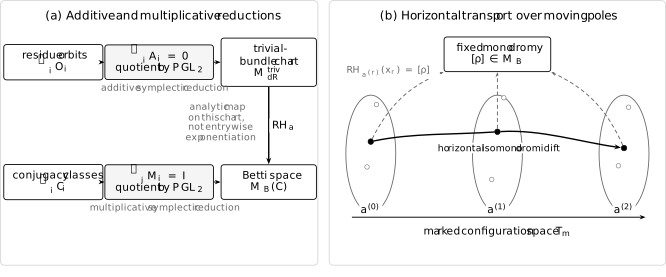
The upper reduction produces the trivial-bundle de Rham residue chart; the full stable-parabolic moduli problem can contain additional bundle strata. That chart and the Betti space are joined by the restricted analytic Riemann–Hilbert map. As the marked poles move, an isomonodromic leaf crosses the de Rham fibers while every point on it maps to one fixed Betti point. The dimensions are schematic, and no global triviality over configuration space is implied.

Dimension counting and the rigid three-pole checkpoint

For a noncentral semisimple element of $\mathfrak{sl}_2$, the adjoint orbit has complex dimension two. At an irreducible transverse tuple,

$$\begin{aligned} \dim_{\mathbb C} \mathcal M_{\mathrm{dR}} (\boldsymbol a,\boldsymbol\theta) &= \underbrace{2m}_{\text{residue orbits}} - \underbrace{3}_{\sum A_i=0} - \underbrace{3}_{PGL(2)\text{ quotient}} \\ &= 2m-6. \end{aligned}$$

The same count holds for the relative Betti space: the product relation has rank three, and simultaneous conjugation removes three effective directions. The stabilizer of an irreducible $SL(2)$ tuple is the center $\{\pm I\}$, but irreducibility alone does not replace the transversality and noncentral-class hypotheses.

Adding the position base gives

$$\begin{aligned} \dim_{\mathbb C}\mathcal T_m &= m-3, \\ \dim_{\mathbb C}\mathfrak M_{\mathrm{dR}} (\boldsymbol\theta) &= 3m-9. \end{aligned}$$

The first three cases explain the special-function hierarchy:

Number of poles	Phase dimension	Time dimension	Generic model
$m=3$	$0$	$0$	Rigid hypergeometric-type system
$m=4$	$2$	$1$	Painlevé VI phase space
$m=5$	$4$	$2$	Two-time Garnier system

The total $m=4$ family has complex dimension three, so it cannot itself be a symplectic manifold. What it carries is a family of symplectic two-dimensional fibers together with an isomonodromic horizontal connection.

Exact three-pole residue model

The zero-dimensional count can be audited directly. Diagonalize one residue and write

$$A_0 = \begin{pmatrix} \alpha&0\\ 0&-\alpha \end{pmatrix}, \qquad A_1 = \begin{pmatrix} b&c\\ d&-b \end{pmatrix}.$$

If the spectra of $A_0,A_1,A_\infty=-A_0-A_1$ are $\{\pm\alpha\}$, $\{\pm\beta\}$, and $\{\pm\gamma\}$, respectively, then

$$\begin{aligned} b^2+cd &= \beta^2, \\ (\alpha+b)^2+cd &= \gamma^2. \end{aligned}$$

For $\alpha\neq0$,

$$b = \frac{ \gamma^2-\beta^2-\alpha^2 }{ 2\alpha }, \qquad cd = \beta^2-b^2.$$

When $cd\neq0$, residual diagonal conjugation removes the remaining split between $c$ and $d$. The tuple is therefore unique up to conjugation on this generic chart.

Choose

$$\alpha=\frac14, \qquad \beta=\frac13, \qquad \gamma=\frac14.$$

Then

$$b=-\frac29, \qquad cd=\frac5{81},$$

and one representative is

$$\begin{aligned} A_0 &= \begin{pmatrix} 1/4&0\\ 0&-1/4 \end{pmatrix}, \\ A_1 &= \begin{pmatrix} -2/9&1\\ 5/81&2/9 \end{pmatrix}, \\ A_\infty &= \begin{pmatrix} -1/36&-1\\ -5/81&1/36 \end{pmatrix}. \end{aligned}$$

The spectra are exactly

$$\operatorname{spec}(A_0,A_1,A_\infty) = \left( \left\{\pm\frac14\right\}, \left\{\pm\frac13\right\}, \left\{\pm\frac14\right\} \right).$$

Neither coordinate eigenline of $A_0$ is preserved by $A_1$, so the additive tuple has no common invariant line. Its exponent differences and local monodromy traces are

$$\begin{aligned} (\theta_0,\theta_1,\theta_\infty) &= \left( \frac12,\frac23,\frac12 \right), \\ (\kappa_0,\kappa_1,\kappa_\infty) &= \left( 0,-1,0 \right). \end{aligned}$$

For a three-puncture $SL(2)$ character, reducibility would force

$$\kappa_0^2+\kappa_1^2+\kappa_\infty^2 - \kappa_0\kappa_1\kappa_\infty - 4 = 0.$$

The present value is $-3$, so the corresponding Betti character is irreducible; with these noncentral semisimple classes, it supplies the intended good-locus checkpoint. These traces still do not claim that the based monodromy matrices are the three residue exponentials: the global connection matrices are required.

Isomonodromy is horizontal transport

Let $U\subset\mathcal T_m$ be a simply connected marking chamber. Choose a base point in the punctured sphere, distinguished loops, and an isotopy that transports them as the punctures move. Over $U$, the Betti family is then topologically trivialized, and the relative Riemann–Hilbert map has the local form

$$\begin{array}{ccc} \mathfrak M_{\mathrm{dR}} (\boldsymbol\theta)|_U & \xrightarrow{\ \operatorname{RH}\ } & U\times \mathcal M_{\mathrm B}(\boldsymbol{\mathcal C}) \\ \downarrow && \downarrow \\ U&=&U. \end{array}$$

For one Betti point $[\rho]$, define

$$\mathcal L_{[\rho]} = \operatorname{RH}^{-1} \left( U\times\{[\rho]\} \right).$$

On the good locus this is a local horizontal leaf of dimension $m-3$, intersecting each nearby fixed-time de Rham fiber in one point. Along it, the following ledger applies:

Held fixed	Allowed to move
Full marked representation class $[\rho]$	Pole positions $\boldsymbol a$
Local exponent lifts in the chosen Schlesinger chart	Residue matrices and accessory coordinates
Determinant, loop, and lift conventions	ODE connection coefficients tied to external normalizations, unless included in the declared framed datum
Declared tame or wild monodromy data	Possibly the bundle splitting on an exceptional divisor

The qualification in the third row matters. A coarse Betti point does not determine every coefficient between independently normalized local ODE bases. In a framed Jimbo–Miwa–Ueno problem, however, the declared local-to-global connection matrices are themselves part of the generalized monodromy data and are held fixed.

An extended flat system realizes the horizontal lift:

$$\dd Y = \left[ A(z,\boldsymbol a)\,\dd z + \sum_r B_r(z,\boldsymbol a)\,\dd a_r \right]Y.$$

Writing its curvature as $\dd\Omega-\Omega\wedge\Omega=0$ gives

$$\frac{\partial A}{\partial a_r} - \frac{\partial B_r}{\partial z} + [A,B_r] = 0.$$

The next page chooses the Fuchsian $B_r$ and derives the Schlesinger equations. At this stage, flatness is the mechanism and “fixed marked monodromy” is the geometric definition.

A marking is part of “constant monodromy”

The fundamental groups for different pole configurations are identified only after the loops have been transported. If the positions follow a closed braid, resetting to a standard generator system can act on the monodromy tuple by a mapping-class transformation. With one standard orientation, an adjacent Hurwitz move is

$$(M_i,M_{i+1}) \longmapsto \left( M_{i+1}, M_{i+1}^{-1}M_iM_{i+1} \right),$$

which preserves the ordered product $M_iM_{i+1}$. The inverse braid uses the inverse move; closed loops of labeled configurations give pure-braid composites.

Thus matrices can be literally constant on the universal cover of configuration space, or in a continuously transported marking. They need not have identical entries after a global loop followed by a reset of the standard cuts.

Four true poles produce one time and two phase coordinates

Rename Chapter 3’s cross-ratio $a$ as the deformation time $t$, and list the same normalized four-point set as $0,t,1,\infty$:

$$A(z;t) = \frac{A_0(t)}z + \frac{A_t(t)}{z-t} + \frac{A_1(t)}{z-1}, \qquad A_\infty = -A_0-A_t-A_1.$$

The base coordinate

$$t\in \mathbb P^1\setminus\{0,1,\infty\}$$

is the single deformation time. Each fixed-$t$ de Rham fiber is a complex surface. Darboux coordinates $(q,p)$ describe its moving phase point, whereas a pair-trace parameter such as

$$\operatorname{tr}(M_0M_t) = 2\cos(\pi\sigma)$$

and a conjugate twist coordinate supply two convention-dependent Betti coordinates. The local traces $\kappa_\nu$ and the Betti coordinates remain constant along an isomonodromic leaf; $q(t)$ and $p(t)$ evolve. Their Hamiltonian interpretation is developed two pages ahead.

Preview lemma: scalar projection creates an apparent pole

Write the system coefficient as

$$A(z) = \begin{pmatrix} a(z)&b(z)\\ c(z)&-a(z) \end{pmatrix}.$$

If $u$ is the first component of $Y$, eliminating the second component where $b\neq0$ gives

$$u'' - \frac{b'}b\,u' - \left( a'+a^2+bc-a\frac{b'}b \right)u = 0.$$

After diagonalizing $A_\infty$, the upper-right residue at infinity vanishes. If $b_0,b_t,b_1$ are the upper-right entries of the three finite residues, then

$$b_0+b_t+b_1=0$$

and

$$\begin{aligned} b(z) &= \frac{b_0}{z} + \frac{b_t}{z-t} + \frac{b_1}{z-1} \\ &= -\frac{\chi(z-q)} {z(z-1)(z-t)}, \\ \chi &= t b_0+(t-1)b_1, \qquad q = \frac{t b_0}{\chi}. \end{aligned}$$

This chart assumes $\chi\neq0$ and that $q$ does not collide with a true pole. At a simple zero $z=q$ of $b$, the system itself is ordinary, while the scalar equation has

$$-\frac{b'}b = -\frac1{z-q}+O(1).$$

There is no double pole in the scalar potential term, so the indicial equation is

$$\rho(\rho-1)-\rho = \rho(\rho-2) = 0.$$

The exponents are $0$ and $2$, and the singularity has trivial local monodromy because both scalar solutions come from an analytic system. It is an apparent singularity, and its moving position $q(t)$ becomes the Painlevé VI coordinate.

This is why a generic four-pole Painlevé VI Lax system is not literally a four-singularity Heun equation after scalar reduction: it normally has an additional apparent pole. Heun reductions arise on special slices, after apparent-pole constraints, or through the tau/accessory relations developed later in the chapter. Page 5 takes this lemma as input rather than repeating it; its new task is to derive the actual specialization and tau/accessory constraints that remove or control the apparent pole.

Meromorphic connections with irregular poles

The residue model is the tame, logarithmic sector of a broader meromorphic theory. At an irregular pole, ordinary loop monodromy is not the complete datum. A formal solution has the schematic form

$$\widehat Y_i(w) = \widehat G_i(w) \exp Q_i(w) w^{\Lambda_i},$$

with a local ramified coordinate understood when necessary. Its deformation ledger separates three roles:

Role	Irregular data
Moving times	Selected coefficients of the nonlogarithmic exponential polynomial $Q_i$, and possibly pole positions
Fixed combinatorial type within one chart	Pole order, ramification, exponential labels, and a transported Stokes-sector ordering
Fixed generalized monodromy invariants	Formal monodromy exponent $\Lambda_i$, transported direction-labeled Stokes factors, and normalized sectorial-to-global connection matrices

Thus the irregular type $Q_i$ is part of the formal normal form but its selected coefficients are deformation variables, not conserved monodromy invariants. Isomonodromy preserves the last row while those times and the ODE coefficient matrices move. A direction collision or change of Stokes combinatorics can require a new chart. The precise factorization and its ordering conventions were established on the wild-monodromy page; Chapter 5 returns to them during confluence.

Route through the chapter

Page	New layer	Main safeguard
1. Connections and monodromy moduli	De Rham fibers, Betti space, and horizontal leaves	Fixed-time phase space is not the isomonodromic leaf
2. Lax compatibility and Schlesinger equations	Differential equations for horizontal lift	Flatness and sign conventions are derived
3. Hamiltonian structure and accessory parameters	Darboux coordinates and Hamiltonians	Time, phase, and monodromy coordinates stay distinct
4. Jimbo–Miwa–Ueno tau functions	Closed deformation one-form	Tau normalization and zero loci are qualified
5. Painlevé Lax systems and Heun reductions	Scalar reduction and apparent-pole constraints	Generic Painlevé VI is not identified with generic Heun
6. Confluence through Painlevé V, III, IV, and II	Wild times and limiting systems	$P_{\mathrm{III}}(D_6)$, $P_{\mathrm{III}}(D_7)$, and $P_{\mathrm{III}}(D_8)$ remain distinct
7. Inverse monodromy and spectral constraints	Boundary data select monodromy loci	A tau zero is not automatically a spectrum
8. Series, Fredholm formulae, and numerics	Reproducible evaluation	Isomonodromic and scalar spectral determinants are distinct

Common pitfalls

Exponentiating every residue in the global frame. A residue exponential describes local monodromy only in an adapted nonresonant local frame. Connection matrices transport those local matrices to one based global frame, and they depend on the whole connection.

Calling the residue quotient the complete moduli space. The displayed tuple quotient is a powerful trivial-bundle chart. A global de Rham point also knows the logarithmic bundle, determinant structure, extension or parabolic data, and stability condition.

Saying “monodromy is constant” without a marking. The representation is constant after Gauss–Manin transport of the base point and loops. Around a closed path in configuration space, a standard tuple can return after a nontrivial braid or mapping-class transformation.

Confusing horizontal and symplectic leaves. Fixed local conjugacy classes select a symplectic leaf on the Betti side, and each fixed-time de Rham fiber is symplectic on the good locus. An isomonodromic leaf instead crosses those fibers and maps to a single Betti point.

Equating Painlevé VI with Heun. Painlevé VI governs the motion of a four-pole Lax system with fixed monodromy. Generic scalar reduction adds a moving apparent singularity; obtaining a Heun equation requires an additional reduction, specialization, or tau/accessory constraint.

Preserving only ordinary monodromy at an irregular pole. The ordinary product forgets the direction-labeled Stokes factorization. A wild isomonodromic problem must state exactly which formal, Stokes, ramification, and connection data are held fixed.

Exercises

1. From residue exponents to local traces

Let $A_i$ have eigenvalues $\pm\theta_i/2$. On a nonresonant local chart, derive the eigenvalues and trace of its local monodromy. Explain what survives when $\theta_i\in\mathbb Z$ and what can fail.

Solution

In an adapted nonresonant frame,

$$D_i = \exp \left[ 2\pi\ii \begin{pmatrix} \theta_i/2&0\\ 0&-\theta_i/2 \end{pmatrix} \right].$$

Therefore

$$\operatorname{spec}D_i = \left\{ \ee^{\pi\ii\theta_i}, \ee^{-\pi\ii\theta_i} \right\}, \qquad \operatorname{tr}D_i = 2\cos(\pi\theta_i).$$

Conjugating to a based frame preserves the spectrum and trace. When $\theta_i\in\mathbb Z$, the eigenvalues still coincide at $1$ or $-1$, so the trace formula survives. The residue orbit alone need not determine the Jordan class: resonant terms can produce logarithmic solutions and a nontrivial unipotent factor multiplying $I$ or $-I$. Monodromy also cannot recover which integer lift of the exponents was chosen.

2. Audit every dimension

Assume $m$ noncentral semisimple residue orbits, an irreducible tuple, and transverse constraints. Derive the dimensions of the de Rham fiber, the configuration base, the total family, and one isomonodromic leaf. Evaluate all four for $m=4$.

Solution

Each $SL(2)$ residue orbit has dimension two, so the product has dimension $2m$. The additive moment-map condition has rank three, and the effective $PGL(2)$ quotient removes three more dimensions:

$$\dim\mathcal M_{\mathrm{dR}} = 2m-3-3 = 2m-6.$$

Three labeled points can be fixed by a Möbius map, leaving

$$\dim\mathcal T_m=m-3.$$

Consequently,

$$\dim\mathfrak M_{\mathrm{dR}} = (2m-6)+(m-3) = 3m-9.$$

A good-locus horizontal leaf contains one point in each nearby fiber, so its dimension equals the time-base dimension $m-3$. For $m=4$, these dimensions are respectively

$$2,\qquad 1,\qquad 3,\qquad 1.$$

3. Verify the rigid residue model

For

$$A_0 = \begin{pmatrix} 1/4&0\\ 0&-1/4 \end{pmatrix}, \qquad A_1 = \begin{pmatrix} -2/9&1\\ 5/81&2/9 \end{pmatrix},$$

compute $A_\infty$, all three spectra, and the local trace triple. Prove that $A_0$ and $A_1$ have no common invariant line, and verify that the three-puncture Betti character is irreducible.

Solution

The residue at infinity is

$$A_\infty = -A_0-A_1 = \begin{pmatrix} -1/36&-1\\ -5/81&1/36 \end{pmatrix}.$$

For a traceless $2\times2$ matrix, the squared eigenvalue is $-\det A$. Here

$$\begin{aligned} -\det A_0&=\frac1{16},\\ -\det A_1&=\frac1{9},\\ -\det A_\infty &= \frac1{16}. \end{aligned}$$

Thus the spectra are

$$\left\{\pm\frac14\right\}, \qquad \left\{\pm\frac13\right\}, \qquad \left\{\pm\frac14\right\}.$$

The exponent differences are $1/2$, $2/3$, and $1/2$, so

$$\left( 2\cos\frac\pi2, 2\cos\frac{2\pi}3, 2\cos\frac\pi2 \right) = (0,-1,0).$$

Because $A_0$ has distinct eigenvalues, any common invariant line would have to be one of the two coordinate axes. But $A_1$ sends each coordinate axis to a vector with both components nonzero, so neither is invariant. Finally,

$$0^2+(-1)^2+0^2-(0)(-1)(0)-4 = -3\neq0.$$

The three-puncture reducibility polynomial does not vanish, so the Betti character is irreducible.

4. Separate local and based monodromy

Suppose the $i$th local frame has monodromy $D_i$ and is related to the continued base frame by a constant connection matrix $C_{*i}$. Derive the based matrix $M_i$. Explain why changing the base frame and changing the local eigenbasis have different effects.

Solution

With the book convention, transport from the local frame to the base frame gives

$$M_i = C_{*i}D_iC_{*i}^{-1}.$$

Changing the base frame by one matrix $H$ simultaneously conjugates every based monodromy matrix:

$$M_i\longmapsto H^{-1}M_iH.$$

Changing only the $i$th local eigenbasis conjugates $D_i$ and changes $C_{*i}$ by the compensating factor, leaving $M_i$ unchanged. Thus a base-point framing is one global choice, whereas local eigenbases are puncture-by-puncture normalizations with their own centralizer freedom.

5. Check a Hurwitz move

Show that

$$(M_i,M_{i+1}) \longmapsto \left( M_{i+1}, M_{i+1}^{-1}M_iM_{i+1} \right)$$

preserves the ordered product. Why does this not contradict isomonodromy?

Solution

The transformed product is

$$M_{i+1} \left( M_{i+1}^{-1}M_iM_{i+1} \right) = M_iM_{i+1}.$$

The move changes the standard generator system after braiding punctures; it does not change the underlying transported local system. Isomonodromy says that the representation is constant under the chosen topological identification. If one resets the loops after a global motion, the matrices are re-expressed through the corresponding mapping-class action.

6. Linearize the multiplicative constraint

Let

$$M_i(\varepsilon) = \exp(2\pi\ii\varepsilon A_i) +O(\varepsilon^2)$$

with $M_1\cdots M_m=I$. Show that the first-order constraint is $\sum_iA_i=0$. Why is this not a proof that $\operatorname{RH}$ is entrywise exponentiation?

Solution

Expanding each factor gives

$$M_i(\varepsilon) = I+2\pi\ii\varepsilon A_i +O(\varepsilon^2).$$

Multiplying in order,

$$M_1\cdots M_m = I +2\pi\ii\varepsilon \sum_iA_i +O(\varepsilon^2).$$

Equality with $I$ forces $\sum_iA_i=0$ at first order. This calculation only identifies the tangent of a group-valued moment-map constraint near the identity. For a finite connection, the based $M_i$ also contain global parallel transport and connection matrices, and noncommutative higher-order terms couple all residues and positions.

7. Derive the apparent singularity

Starting from

$$\begin{aligned} u'&=au+bv,\\ v'&=cu-av, \end{aligned}$$

eliminate $v$. If $b$ has a simple zero at an ordinary system point $q$, derive the scalar indicial roots. For the four-pole coefficient with diagonal $A_\infty$, derive the displayed formula for $q$.

Solution

Where $b\neq0$,

$$v=\frac{u'-au}{b}.$$

Differentiation followed by substitution of $v'$ gives

$$u'' - \frac{b'}b\,u' - \left( a'+a^2+bc-a\frac{b'}b \right)u = 0.$$

If $b(z)=\beta(z-q)+O((z-q)^2)$ with $\beta\neq0$, then the coefficient of $u'$ has residue $-1$, while the coefficient of $u$ has at most a simple pole. Hence

$$\rho(\rho-1)-\rho=0,$$

with roots $0$ and $2$. Since the original matrix system is analytic at $q$, its two solution columns are single-valued there; the induced scalar singularity is apparent.

For

$$b(z) = \frac{b_0}{z} + \frac{b_t}{z-t} + \frac{b_1}{z-1},$$

diagonal $A_\infty$ implies $b_0+b_t+b_1=0$. Combining denominators leaves a linear numerator:

$$b(z) = -\frac{ \bigl[tb_0+(t-1)b_1\bigr]z-tb_0 }{ z(z-1)(z-t) }.$$

Therefore

$$q = \frac{tb_0}{tb_0+(t-1)b_1},$$

provided the denominator is nonzero.

References

• M. Jimbo, T. Miwa, and K. Ueno, “Monodromy Preserving Deformation of Linear Ordinary Differential Equations with Rational Coefficients I: General Theory and $\tau$-Function”, Physica D 2 (1981), 306–352, develops the general compatibility framework and generalized monodromy data.
• K. Iwasaki, H. Kimura, S. Shimomura, and M. Yoshida, From Gauss to Painlevé: A Modern Theory of Special Functions, Vieweg, 1991, develops monodromy-preserving deformation from rigid Fuchsian systems to Painlevé and Garnier equations.
• M. Inaba, K. Iwasaki, and M.-H. Saito, “Moduli of Stable Parabolic Connections, Riemann–Hilbert Correspondence and Geometry of Painlevé Equation of Type VI, Part I”, Publications of the Research Institute for Mathematical Sciences 42 (2006), 987–1089, constructs the stable-parabolic moduli spaces and proves the qualified global Riemann–Hilbert and symplectic-resolution statements used here.
• P. P. Boalch, “Symplectic Manifolds and Isomonodromic Deformations”, Advances in Mathematics 163 (2001), 137–205, gives an intrinsic symplectic account of tame and irregular isomonodromic deformation.
• W. M. Goldman, “The Symplectic Nature of Fundamental Groups of Surfaces”, Advances in Mathematics 54 (1984), 200–225, constructs the representation-space symplectic form from cohomology, cup product, and the invariant pairing.
• A. Alekseev, A. Malkin, and E. Meinrenken, “Lie Group Valued Moment Maps”, Journal of Differential Geometry 48 (1998), 445–495, develops the quasi-Hamiltonian reduction that realizes character varieties as multiplicative symplectic quotients.
• P. Deligne, Équations différentielles à points singuliers réguliers, Lecture Notes in Mathematics 163, Springer, 1970, supplies the logarithmic extension and regular-singular Riemann–Hilbert background.
• K. Iwasaki, “Fuchsian Moduli on a Riemann Surface—Its Poisson Structure and Poincaré–Lefschetz Duality”, Pacific Journal of Mathematics 155 (1992), 319–340, treats Fuchsian moduli, their Poisson structure, and the parabolic-cohomology pairing.

What the page has established

At fixed pole positions, logarithmic connections form a de Rham phase space and monodromy representations form a Betti phase space. The Riemann–Hilbert map relates them analytically on the good locus. Isomonodromy is the horizontal lift of a fixed, marked Betti point through the family of de Rham fibers. The next page turns that geometry into the Schlesinger differential equations.