Exact-WKB/GMN-Type Riemann–Hilbert Integral Equations

Page 2 inverted functional relations after choosing analytic strips and spectral divisors. This page begins from different data: Borel-summed Voros symbols, a fixed BPS chamber, and intersection-controlled jumps in the complex semiclassical-parameter plane. The result is a nonlinear Riemann–Hilbert equation whose logarithm looks TBA-like, but whose rays, kernel, discrete input, and output are not those of the ODE/IM equations.

Two normalizations must be kept separate. The full DDP-normalized GMN-type problem has paired asymptotics at $\zeta=0$ and $\zeta=\infty$, an antipodal reality condition, and exponential damping at both ends of every BPS ray. Its conformal limit retains the exact-WKB drive $\exp(Z_\gamma/\hbar)$ and uses an origin-subtracted Cauchy kernel, but its far endpoint requires a new convergence hypothesis. On a distinguished Hitchin section this limit can have an oper interpretation, subject to further assumptions. Page 4 will ask when either construction can be identified with an ODE/IM TBA.

Status ledger

Passage	Status on this page
Ordinary-saddle DDP jump	The Chapter 9 theorem under its stated exact-WKB and summability hypotheses
Charge lattice, BPS indices, and quadratic refinement	Fixed-chamber input; they must be derived separately for a particular ODE
BPS-ray orientation and bank labels	Exact definitions in the book’s convention
Symmetric Cauchy equation from the declared jumps	Exact Plemelj reconstruction under the displayed endpoint, branch, and summability assumptions
Large-$R$ solution by iteration	Available under support, growth, nonvanishing, and contraction bounds; not a general small-$R$ theorem
Finite uncoupled conformal solution	Bridgeland’s theorem assumes an integral uncoupled BPS structure, unit active constant terms, and polynomial growth at infinity
Conformal exact-WKB equation	Conditional on a controlled scaling limit or an independent endpoint estimate
Borel-summed Voros symbols equal cluster coordinates	A theorem in Allegretti’s stated complete saddle-free setting
Borel sums solve a BPS RH problem	Model-specific; Iwaki–Kidwai prove the cited hypergeometric-type uncoupled cases
Equality with ODE/IM TBA	Not asserted; Page 4 supplies the comparison gates
Coincident noncommuting rays and chamber change	Deferred to Page 5

A fixed-chamber passport has independent analytic and discrete data

Let $\Gamma$ be a free abelian charge lattice equipped with an integer-valued skew pairing

$$\gamma\mathbin{\cdot}\rho = -\rho\mathbin{\cdot}\gamma.$$

The central charge is an additive map

$$Z:\Gamma\longrightarrow\mathbb C, \qquad Z_{\gamma+\rho}=Z_\gamma+Z_\rho.$$

In the exact-WKB realization of Chapters 8 and 9,

$$Z_\gamma=\oint_\gamma\lambda_0,$$

where $\gamma$ is an anti-invariant cycle on the normalized WKB cover. This period locates a possible ray; it does not by itself say that the charge is active. Activity is separate integer data

$$\Omega_{\mathrm{BPS}}:\Gamma\longrightarrow\mathbb Z.$$

For the paired, reality-symmetric problem, assume the CPT symmetry

$$\Omega_{\mathrm{BPS}}(-\gamma) = \Omega_{\mathrm{BPS}}(\gamma).$$

The subscript prevents confusion with the all-orders WKB form $\Omega(\hbar)$. A regular saddle connection has the local hypermultiplet calibration $\Omega_{\mathrm{BPS}}=1$. A cylinder, simple-pole wall, loop, or degenerate saddle has different data and must not be inserted into the ordinary-saddle formula by analogy.

The full fixed-chamber passport is

$$\left( \Gamma,\, \mathbin{\cdot},\, Z,\, \Omega_{\mathrm{BPS}},\, \sigma,\, R,\, \vartheta \right).$$

Here $\sigma:\Gamma\to\{\pm1\}$ is a quadratic refinement, $R>0$ is the semiclassical size, and

$$\vartheta:\Gamma \longrightarrow \mathbb R/(2\pi\mathbb Z)$$

is additive, so $\vartheta_{-\gamma}=-\vartheta_\gamma$ modulo $2\pi$. The refinement obeys

$$\begin{aligned} \sigma(\gamma)\sigma(\rho) ={}& (-1)^{\gamma\mathbin{\cdot}\rho} \sigma(\gamma+\rho). \end{aligned}$$

It packages the sign relating ordinary multiplicative coordinates to intrinsic twisted-torus coordinates. Locally, an ordinary saddle is calibrated by $\sigma(\delta)=-1$, which turns $1-\sigma(\delta)\mathcal V_\delta$ into $1+\mathcal V_\delta$. One cannot set $\sigma=-1$ on every active charge of an arbitrary coupled spectrum without checking the quadratic-refinement identity.

For an infinite active set, two controls play different roles. A support property keeps active central charges away from zero relative to charge size,

$$|Z_\delta|\ge c\|\delta\|, \qquad \Omega_{\mathrm{BPS}}(\delta)\ne0,$$

whereas a separate growth condition controls the degeneracies, for example

$$\sum_\delta \left| \Omega_{\mathrm{BPS}}(\delta) \right| \ee^{-R_0|Z_\delta|} <\infty$$

for some $R_0>0$. The first condition does not imply the second. Locally finite rays or a convergent ordered sector product are also needed. Until Page 5, assume distinct active rays, or only mutually local charges on a common ray.

First reading

Take a finite active set with distinct rays, put $\Omega_{\mathrm{BPS}}=1$ on those rays, and use the local ordinary-saddle calibration $\sigma=-1$. The general notation then records exactly which assumptions must be restored for coupled or infinite spectra.

For each $\gamma$, the RH unknown is a nonzero function $\mathcal V_\gamma(\zeta)$, holomorphic on $\mathbb C^\times$ minus the active rays and admitting boundary values on both banks. “Riemann–Hilbert” means that these functions are reconstructed from their prescribed multiplicative jumps together with endpoint asymptotics, a character law, and reality data.

The contrast with Page 2 is structural:

ODE/IM inversion	Exact-WKB/GMN reconstruction
Baxter divisor or finite fusion nodes	Charge lattice and active BPS classes
Multiplicative $q$-shifts	Rays in the $\zeta$-plane
Fusion incidence matrix	Skew intersection pairing
Fourier or Wiener–Hopf inverse	Cauchy or Plemelj inverse
Determinant or pseudoenergy	Resummed period or Darboux coordinate

Central charges determine decay rays, not spatial Stokes curves

For an oriented active charge $\delta$, define its BPS ray by

$$\begin{aligned} \ell_\delta &= \left\{ \zeta: \frac{Z_\delta}{\zeta}\in\mathbb R_{<0} \right\} \\ &= -Z_\delta\mathbb R_{>0}. \end{aligned}$$

This ray lies in the complex $\zeta$-plane. It is not a Stokes curve drawn in the ODE’s spatial $z$-plane. Orient $\ell_\delta$ outward, from $0$ to $\infty$, and define

• the $+$ boundary as the left, counterclockwise bank;
• the $-$ boundary as the right, clockwise bank.

After rotating a ray to the positive real axis, these are exactly the upper and lower banks used in Chapter 9. The 2010 GMN paper instead calls the right bank $+$ and the left bank $-$, so

$$\mathcal V_+^{\mathrm{book}} = \mathcal X_-^{\mathrm{GMN10}}, \qquad \mathcal V_-^{\mathrm{book}} = \mathcal X_+^{\mathrm{GMN10}}.$$

At fixed geometric pairing, the original interaction coefficient is

$$-\frac{ \Omega_{\mathrm{BPS}}(\delta) (\gamma\mathbin{\cdot}\delta) }{ 4\pi\ii } = +\frac{ \Omega_{\mathrm{BPS}}(\delta) (\delta\mathbin{\cdot}\gamma) }{ 4\pi\ii },$$

which is opposite to the coefficient below. Original GMN imposes the clockwise value as a KS transform of the counterclockwise value; Chapter 9 DDP imposes the counterclockwise value as the transform of the clockwise value.

This page also follows the inverse, later-GMN/DDP phase-jump convention; GMN’s 2013 WKB paper explicitly notes the sign change from the earlier paper. Thus the jump is inverted as well as the banks being relabeled. The coefficient below is derived directly from the book’s DDP jump and Plemelj, not copied from the 2010 formula.

Write

$$Z_\delta = |Z_\delta|\ee^{\ii\phi_\delta}, \qquad \zeta' = -\ee^{\ii\phi_\delta}t, \quad t>0.$$

The semiflat coordinate is the jump-free reference coordinate carrying the prescribed endpoint asymptotics. It is

$$\begin{aligned} \mathcal V_\gamma^{\mathrm{sf}}(\zeta) = \exp\!\left[ \pi R \left( \frac{Z_\gamma}{\zeta} +\overline{Z_\gamma}\zeta \right) +\ii\vartheta_\gamma \right]. \end{aligned}$$

On its own ray, the active coordinate has modulus

$$\left| \mathcal V_\delta^{\mathrm{sf}}(\zeta') \right| = \exp\!\left[ -\pi R|Z_\delta| \left( t+t^{-1} \right) \right].$$

It therefore decays exponentially as $t\to0$ and as $t\to\infty$. The first decay is the exact-WKB choice $\operatorname{Re}(Z_\delta/\zeta')<0$; the second comes from the conjugate term and is lost in the conformal limit.

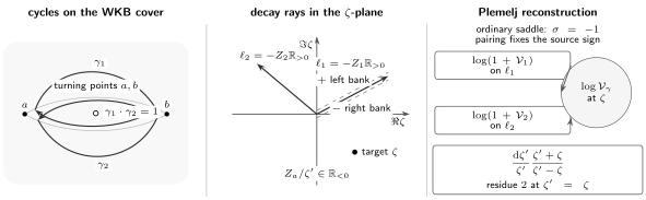
Fixed-chamber Riemann–Hilbert reconstruction. Intersection data decide which ray logarithm acts on each coordinate. The orientation $Z_\delta/\zeta'<0$ makes the active symbol small near the origin, while the full semiflat term also damps the far endpoint. No Baxter divisor, fusion graph, or ODE/IM Fourier kernel enters this construction.

The DDP automorphism supplies the jump

Chapter 9 fixed the active cycle as the first argument of the intersection pairing. In the local ordinary-saddle calibration, the analytic jump across $\ell_\delta$ is

$$\begin{aligned} \mathcal V_{\gamma,+} ={}& \mathcal V_{\gamma,-} \\ &\times \left( 1+\mathcal V_{\delta,-} \right)^{ -\Omega_{\mathrm{BPS}}(\delta)\, \delta\mathbin{\cdot}\gamma }. \end{aligned}$$

For $\Omega_{\mathrm{BPS}}(\delta)=1$, this is precisely the DDP formula already proved in its stated scope. The active coordinate is unchanged because $\delta\mathbin{\cdot}\delta=0$.

The refinement-aware jump is obtained by replacing the logarithmic factor with

$$\Log\!\left( 1-\sigma(\delta)\mathcal V_{\delta,-} \right).$$

Thus the logarithmic boundary difference is

$$\begin{aligned} \Log\mathcal V_{\gamma,+} -\Log\mathcal V_{\gamma,-} ={}& -\Omega_{\mathrm{BPS}}(\delta) \left( \delta\mathbin{\cdot}\gamma \right) \\ &\times \Log\!\left( 1-\sigma(\delta)\mathcal V_{\delta,-} \right). \end{aligned}$$

The branch is continued from a ray endpoint where the active coordinate is small. If $1-\sigma(\delta)\mathcal V_\delta$ vanishes on the contour, that branch prescription fails: the contour must be deformed or supplied with source terms. Those are Page 5 operations.

Phase alignment is not enough to assert this jump. A saddle connection, cylinder, or other justified BPS state must actually realize the charge, and its index must be known. Likewise, aligned noncommuting charges require an ordered product of jump factors rather than one scalar logarithm.

A residue-two Cauchy kernel reconstructs the full coordinate

Introduce the symmetric one-form

$$K(\zeta,\zeta') = \frac{\dd\zeta'}{\zeta'} \frac{\zeta'+\zeta}{\zeta'-\zeta}.$$

Near the target point,

$$K(\zeta,\zeta') = 2\frac{\dd\zeta'}{\zeta'-\zeta} +\text{regular}.$$

Because the residue is $2$, the Plemelj coefficient is $1/(4\pi\ii)$, not $1/(2\pi\ii)$. With every ray oriented $0\to\infty$, the book-normalized equation is

$$\begin{aligned} \Log\mathcal V_\gamma(\zeta) ={}& \Log\mathcal V_\gamma^{\mathrm{sf}}(\zeta) \\ &- \frac{1}{4\pi\ii} \sum_\delta \Omega_{\mathrm{BPS}}(\delta) \left( \delta\mathbin{\cdot}\gamma \right) \\ &\quad\times \int_{\ell_\delta}^{0\to\infty} \frac{\dd\zeta'}{\zeta'} \frac{\zeta'+\zeta}{\zeta'-\zeta} \\ &\quad\times \Log\!\left( 1-\sigma(\delta) \mathcal V_\delta(\zeta') \right). \end{aligned}$$

For a local ordinary saddle, put $\sigma(\delta)=-1$. Taking the left-minus-right boundary value of its integral gives

$$-\Omega_{\mathrm{BPS}}(\delta) \left( \delta\mathbin{\cdot}\gamma \right) \Log(1+\mathcal V_\delta),$$

which is exactly the declared DDP jump. This one-line residue check is the safest way to translate between sources with different bank labels. When the target lies on a ray, the integral means a principal value plus the appropriate half-residue boundary term.

The equation is posed with the character law

$$\mathcal V_{\gamma+\rho} = \mathcal V_\gamma\mathcal V_\rho, \qquad \mathcal V_{-\gamma} = \mathcal V_\gamma^{-1},$$

With the even BPS spectrum, $\sigma(-\delta)=\sigma(\delta)$, and logarithm branches paired by antipodal conjugation, the equation also obeys the reality condition

$$\mathcal V_\gamma(\zeta) = \overline{ \mathcal V_{-\gamma} \left( -\frac1{\overline\zeta} \right) },$$

and the paired asymptotic orders

$$\begin{aligned} \Log\mathcal V_\gamma(\zeta) &= \frac{\pi RZ_\gamma}{\zeta} +O(1), && \zeta\to0, \\ \Log\mathcal V_\gamma(\zeta) &= \pi R\overline{Z_\gamma}\zeta +O(1), && \zeta\to\infty. \end{aligned}$$

The bounded zero mode is part of the normalization. In particular, the symmetric kernel approaches a nonzero constant as $\zeta\to0$; one should not silently strengthen the first line to $\mathcal V_\gamma/\mathcal V_\gamma^{\mathrm{sf}}\to1$.

For a finite spectrum, the semiflat estimate gives endpoint convergence if the nonlinear solution remains controlled relative to the semiflat seed and the logarithm has no contour zero. For an infinite spectrum, charge sums, ray integrals, and limits may be interchanged only under uniform domination. GMN’s large-$R$ Appendix C gives a contraction argument only after its weighted multicover and convergence assumptions, together with the needed uniform bounds, supplement the support estimate. The rigorous theorems cited here cover restricted settings; they do not prove a pole-free global solution for every such spectrum, or at arbitrary small $R$.

The conformal equation changes both the drive and the endpoint problem

To compare the full coordinate with the book’s exact-WKB symbol, set

$$\zeta=\pi R\hbar.$$

Then the semiflat exponent becomes

$$\begin{aligned} \pi R \left( \frac{Z_\gamma}{\zeta} +\overline{Z_\gamma}\zeta \right) ={}& \frac{Z_\gamma}{\hbar} \\ &+ \pi^2R^2 \overline{Z_\gamma}\hbar. \end{aligned}$$

The formal conformal scaling

$$R\to0, \qquad \zeta\to0, \qquad \hbar=\frac{\zeta}{\pi R} \quad\text{fixed}$$

therefore retains the exact-WKB factor $\exp(Z_\gamma/\hbar)$ and removes the conjugate drive. But it also removes the large-$|\hbar'|$ damping along every integration ray. The limit cannot generally be passed under the integral sign.

The kernel identity

$$\begin{aligned} & \frac14 \frac{\dd\zeta'}{\zeta'} \frac{\zeta'+\zeta}{\zeta'-\zeta} \\ &\qquad= \frac14\frac{\dd\zeta'}{\zeta'} + \frac12 \frac{\zeta\,\dd\zeta'}{ \zeta'(\zeta'-\zeta) } \end{aligned}$$

separates a target-independent constant from an origin-normalized Cauchy transform. If the constant is absorbed into a declared zero mode $c_\gamma$, and if the limiting integral converges, one obtains

$$\begin{aligned} \Log\mathcal V_\gamma^{\mathrm{conf}}(\hbar) ={}& \frac{Z_\gamma}{\hbar} +c_\gamma \\ &- \frac{\hbar}{2\pi\ii} \sum_\delta \Omega_{\mathrm{BPS}}(\delta) \left( \delta\mathbin{\cdot}\gamma \right) \\ &\quad\times \int_{\ell_\delta} \frac{\dd\hbar'}{ \hbar'(\hbar'-\hbar) } \\ &\quad\times \Log\!\left( 1-\sigma(\delta) \mathcal V_\delta^{\mathrm{conf}}(\hbar') \right). \end{aligned}$$

Indeed,

$$\frac{\hbar}{ \hbar'(\hbar'-\hbar) } = \frac1{\hbar'-\hbar} -\frac1{\hbar'},$$

so the second term fixes the origin normalization while leaving the jump unchanged. Matching a regularized exact-WKB cycle symbol usually selects $c_\gamma=0$, but only when this book explicitly chooses a regularization whose quantum correction tends to zero. That is normalization data, not a consequence of Plemelj. The zero modes are not independent: the character law requires

$$c_{\gamma+\rho} = c_\gamma+c_\rho \pmod{2\pi\ii}$$

on the declared logarithm branches, with $c_{-\gamma}=-c_\gamma$ modulo the same branch period. Any real section must also impose its inherited conjugation condition.

For each source ray, a direct sufficient endpoint contract is

$$\begin{aligned} & \int_0^\varepsilon \frac{ \left| \Log(1-\sigma(\delta)\mathcal V_\delta^{\mathrm{conf}}) \right| }{ |\hbar'| } \,|\dd\hbar'| <\infty, \\ & \int_A^\infty \frac{ \left| \Log(1-\sigma(\delta)\mathcal V_\delta^{\mathrm{conf}}) \right| }{ |\hbar'|^2 } \,|\dd\hbar'| <\infty. \end{aligned}$$

for some $\varepsilon>0$ and $A>0$ along the ray. The semiclassical exponential controls the first integral. A bounded far-end logarithm already controls the second, so decay is sufficient but not necessary.

Gaiotto’s published conformal equation inherits the original GMN crossing direction and therefore has the opposite interaction sign at fixed geometric pairing. The equation above is its DDP-normalized inverse-jump analogue.

Gaiotto’s conformal scaling assumes that the limit exists and has controlled large-$\hbar$ behavior. Its oper interpretation further restricts to the distinguished section with vanishing Wilson-line angles, up to canonical refinement signs; the general identification of the limiting Lagrangian with the oper locus is conjectural.

Allegretti proves that Borel sums of Voros symbols equal Fock–Goncharov coordinates in the stated complete saddle-free setting, but that theorem alone does not say that they solve the nonlinear equation displayed here. Iwaki–Kidwai give an actual model-specific BPS-RH solution for hypergeometric-type quantum curves and almost-doubled uncoupled BPS structures. Outside such settings, a matching leading exponential and matching jump factor establish a strong analogy—not equality of analytic functions.

Rapidity reveals a phase-shifted Cauchy kernel

The conformal equation can be written in a TBA-like form without turning it into the Page 2 TBA. Put

$$Z_a=m_a\ee^{\ii\phi_a}, \qquad \hbar_a(\theta) = -\ee^{\ii\phi_a-\theta},$$

and define a boundary pseudoenergy by

$$\mathcal V_a(\theta) = \mathcal V_{\gamma_a,-}^{\mathrm{conf}} \bigl( \hbar_a(\theta) \bigr) = \ee^{-\varepsilon_a(\theta)}.$$

Then $Z_a/\hbar_a=-m_a\ee^\theta$. Parameterizing the source ray in the same way gives

$$\begin{aligned} \frac{\hbar_a(\theta)}{ \hbar_b(\theta')-\hbar_a(\theta) } = \frac1{ \exp[ \theta-\theta' +\ii(\phi_b-\phi_a) ]-1 }. \end{aligned}$$

Thus the origin-normalized equation has the schematic form

$$\begin{aligned} \varepsilon_a(\theta) ={}& m_a\ee^\theta-c_a \\ &+ \frac1{2\pi\ii} \sum_b \Omega_{\mathrm{BPS}}(\gamma_b) \left( \gamma_b\mathbin{\cdot}\gamma_a \right) \\ &\quad\times \int_{\mathbb R} \frac{ L_b(\theta')\,\dd\theta' }{ \ee^{ \theta-\theta' +\ii(\phi_b-\phi_a) }-1 }, \end{aligned}$$

with

$$L_b = \Log\!\left( 1-\sigma(\gamma_b) \ee^{-\varepsilon_b} \right).$$

The kernel comes from relative ray phases. A pole reaches the real integration line when two interacting rays coincide, precisely where the simple fixed-ray factorization ceases to be sufficient. By contrast, Page 2’s kernels came from $q$-shift multipliers and a fusion incidence matrix. Combining antipodal rays can turn the Cauchy kernel into familiar hyperbolic kernels in special models; Page 4 audits the extra identifications required.

Rank two separates exact solvability from nonlinear coupling

First take

$$\Gamma = \mathbb Z\delta\oplus\mathbb Z\beta, \qquad \delta\mathbin{\cdot}\beta=1,$$

with only $\pm\delta$ active and $\Omega_{\mathrm{BPS}}(\pm\delta)=1$. Choose $\sigma(\delta)=\sigma(-\delta)=-1$. The active spectrum is uncoupled because its active charges pair trivially with one another. Consequently,

$$\mathcal V_{\pm\delta} = \mathcal V_{\pm\delta}^{\mathrm{sf}}.$$

The probe coordinate is nevertheless nontrivial:

$$\begin{aligned} \Log \frac{\mathcal V_\beta}{ \mathcal V_\beta^{\mathrm{sf}} } ={}& -\frac1{4\pi\ii} \int_{\ell_\delta} K(\zeta,\zeta') \Log(1+\mathcal V_\delta^{\mathrm{sf}}) \\ &+ \frac1{4\pi\ii} \int_{\ell_{-\delta}} K(\zeta,\zeta') \Log(1+\mathcal V_{-\delta}^{\mathrm{sf}}). \end{aligned}$$

Both integrals converge exponentially, and $|\mathcal V_{\pm\delta}^{\mathrm{sf}}|<1$ on their own rays, so the principal logarithms meet no zero. This is the elementary calibration of an exact finite mutually local solution of the displayed two-ended equation. Bridgeland’s finite uncoupled theorem is a separate result in his one-ended DT normalization and assumes a constant term equal to one on every active class.

Now choose two charges with

$$\gamma_1\mathbin{\cdot}\gamma_2=1, \qquad \Omega_{\mathrm{BPS}}(\gamma_1) = \Omega_{\mathrm{BPS}}(\gamma_2) =1.$$

In one ray half-plane, write $[\Delta_a\Log\mathcal V_b]_{\ell_a}$ for the contribution from $\ell_a$ alone; the antipodal rays must still be added in the full reality-symmetric problem. The ordinary-saddle source terms are

$$\begin{aligned} [\Delta_2\Log\mathcal V_1]_{\ell_2} &= \frac1{4\pi\ii} \int_{\ell_2} K\Log(1+\mathcal V_2), \\ [\Delta_1\Log\mathcal V_2]_{\ell_1} &= - \frac1{4\pi\ii} \int_{\ell_1} K\Log(1+\mathcal V_1). \end{aligned}$$

The opposite signs are forced by antisymmetry. Iterating these equations produces powers such as $\exp(nZ_{\gamma_a}/\zeta)$ from the Taylor series of $\Log(1+\mathcal V_{\gamma_a})$. They are composite action grades; they do not declare that every multiple $n\gamma_a$ has a nonzero BPS index.

Plemelj equivalence is not a general existence theorem

Under the stated trace and convergence hypotheses, taking boundary values of the integral equation reproduces the jump. Conversely, suppose an RH solution with the declared functional jump law and normalization already exists. Its boundary traces determine actual additive discontinuity functions. Subtract the Cauchy reconstruction of those fixed functions. The logarithmic difference has no jumps, is removable at the two endpoints under the normalization bounds, and vanishes after the zero mode has been fixed. A Liouville argument on the compactified plane then makes the difference zero.

That proves reversibility for an existing solution. It does not prove that the nonlinear fixed-point problem has a solution, that Picard iteration converges, or that no extra poles appear. GMN’s Appendix C gives an argument under additional weighted multicover and convergence assumptions; Garza proves a theorem for a restricted local rank-two setting. General coupled or small-$R$ existence and uniqueness remain model-dependent.

Finally, an RH solution gives resummed cycle or transport coordinates, not an ODE spectrum by itself. A boundary determinant or exact quantization condition must still turn those coordinates into spectral zeros. Page 4 asks when the RH coordinates and the ODE/IM unknowns describe the same analytic objects; Page 5 changes rays, contours, and chamber data.

Common pitfalls

Confusing spatial and parameter-space rays. A Stokes curve lives in the ODE’s $z$-plane. A BPS integration ray lives in the $\zeta$- or $\hbar$-plane and is fixed by a central charge.

Inferring activity from phase alone. The phase of $Z_\delta$ locates a possible ray. A realized saddle class or other justified BPS input is needed to set $\Omega_{\mathrm{BPS}}(\delta)$.

Reversing an intersection or a bank. The book puts the active class first in $\delta\mathbin{\cdot}\gamma$ and calls the left bank $+$. Reversing either convention reverses the exponent; copying a source formula without translating both can hide two sign changes.

Putting a plus sign on every charge. The factor $1+\mathcal V_\delta$ is the local $\sigma(\delta)=-1$ ordinary-saddle calibration. A coupled spectrum must satisfy one coherent quadratic-refinement convention.

Taking the conformal limit under the integral sign. Removing the conjugate drive removes far-end damping. A subtraction changes the normalization, not the missing endpoint estimate.

Calling a fixed-point equation a solution theorem. Plemelj fixes the jump and, with a vanishing condition, its reconstruction. Global nonlinear existence needs a separate contraction, explicit formula, or model-specific theorem.

Recognizing a familiar hyperbolic kernel. Combining antipodal Cauchy rays can produce $1/\cosh$-type kernels. That resemblance does not identify the nodes, masses, unknowns, or observable with ODE/IM; Page 4 requires the complete dictionary.

Changing chamber data inside the equation. The active indices, ray ordering, and refinement package are fixed on this page. Reordering noncommuting rays or changing indices is the wall-crossing problem of Page 5.

Exercises

1. Orient a two-ended decay ray

Let $Z_\delta=|Z_\delta|\ee^{\ii\phi}$ and $\zeta'=-\ee^{\ii\phi}t$. Evaluate the two terms in the semiflat exponent.

Solution

Direct substitution gives

$$\frac{Z_\delta}{\zeta'} = -\frac{|Z_\delta|}{t}, \qquad \overline{Z_\delta}\zeta' = -|Z_\delta|t.$$

Therefore

$$\left| \mathcal V_\delta^{\mathrm{sf}}(\zeta') \right| = \ee^{-\pi R|Z_\delta|(t+t^{-1})}.$$

It decays faster than any power at both endpoints against the measure $\dd t/t$. The conformal limit deletes the term proportional to $t$.

2. Calibrate the Cauchy coefficient

Expand $K(\zeta,\zeta')$ near $\zeta'=\zeta$ and derive the left-minus-right jump produced by one source charge.

Solution

Since $\zeta'/\zeta'=1$ at the pole,

$$K(\zeta,\zeta') = 2\frac{\dd\zeta'}{\zeta'-\zeta} +O(1)\dd\zeta'.$$

The oriented Plemelj formula assigns jump $f$ to $(2\pi\ii)^{-1}\int f(\zeta')\dd\zeta'/(\zeta'-\zeta)$. Hence

$$-\frac{A}{4\pi\ii} \int K\,L$$

has left-minus-right jump $-A L$. Taking $A=\Omega_{\mathrm{BPS}}(\delta) (\delta\mathbin{\cdot}\gamma)$ reproduces the DDP exponent.

3. Compare the two normalizations

Show that the symmetric and origin-normalized kernel one-forms have the same pole and differ by a target-independent term.

Solution

Algebra gives

$$\begin{aligned} & \frac12 \frac{\dd\zeta'}{\zeta'} \frac{\zeta'+\zeta}{\zeta'-\zeta} - \frac{\zeta\,\dd\zeta'}{ \zeta'(\zeta'-\zeta) } \\ &\qquad= \frac{\dd\zeta'}{2\zeta'}. \end{aligned}$$

The difference has no target $\zeta$, so both kernels encode the same Plemelj jump. Their integrals differ by a bounded zero mode, which must be included in the RH normalization.

4. Derive the rank-two signs

Assume $\gamma_1\mathbin{\cdot}\gamma_2=1$. Determine the contribution of $\ell_2$ to $\Log\mathcal V_1$ and of $\ell_1$ to $\Log\mathcal V_2$.

Solution

For target $\gamma_1$, the active-first pairing is

$$\gamma_2\mathbin{\cdot}\gamma_1=-1,$$

so the minus sign in front of the Cauchy sum makes the contribution positive. For target $\gamma_2$, $\gamma_1\mathbin{\cdot}\gamma_2=1$, so the contribution is negative. Self-couplings vanish by skew-symmetry.

5. Find the opposite-charge probe jump

In the uncoupled example, determine the jumps of $\mathcal V_\beta$ on $\ell_\delta$ and $\ell_{-\delta}$.

Solution

Because $\delta\mathbin{\cdot}\beta=1$,

$$\mathcal V_{\beta,+} = \frac{\mathcal V_{\beta,-}}{ 1+\mathcal V_\delta } \qquad\text{on }\ell_\delta.$$

But $(-\delta)\mathbin{\cdot}\beta=-1$, so

$$\mathcal V_{\beta,+} = \mathcal V_{\beta,-} \left( 1+\mathcal V_{-\delta} \right) \qquad\text{on }\ell_{-\delta}.$$

These are exactly the two boundary jumps of the explicit probe Cauchy transform.

6. Derive the phase-shifted rapidity kernel

Substitute $\hbar_a=-\ee^{\ii\phi_a-\theta}$ and $\hbar_b'=-\ee^{\ii\phi_b-\theta'}$ into the origin-normalized Cauchy kernel. Determine when its pole lies on the real $\theta'$-contour.

Solution

The ratio in the kernel is

$$\begin{aligned} \frac{\hbar_a}{ \hbar_b'-\hbar_a } &= \frac1{ \ee^{ \theta-\theta' +\ii(\phi_b-\phi_a) }-1 } \\ &=: K_{ab}(\theta-\theta'). \end{aligned}$$

The parameterization reverses the ray limits, while $\dd\hbar_b'/\hbar_b'=-\dd\theta'$, so the two signs cancel. A pole on the real contour requires

$$\theta-\theta' +\ii(\phi_b-\phi_a) = 2\pi\ii n.$$

For real $\theta,\theta'$, this occurs precisely when $\phi_b-\phi_a=0$ modulo $2\pi$: the two interacting rays coincide. The ordered-product treatment then belongs to Page 5.

As an optional large-$R$ check, let $a>0$, $|\xi|=1$, and define $K_0$ as the modified Bessel function of the second kind. Expanding the logarithm gives

$$\begin{aligned} & \int_0^\infty \frac{\dd t}{t} \Log\!\left( 1+\xi\ee^{-a(t+t^{-1})} \right) \\ &\qquad= 2\sum_{n=1}^\infty \frac{(-1)^{n+1}\xi^n}{n} K_0(2an). \end{aligned}$$

Indeed, $t+t^{-1}\ge2$ makes the logarithmic expansion uniformly dominated, and

$$\int_0^\infty \frac{\dd t}{t} \ee^{-an(t+t^{-1})} = 2K_0(2an).$$

This also quantifies the large-$R$ exponential suppression.

7. Diagnose the naive conformal limit

Use $\zeta=\pi R\hbar$ to find the limiting drive and explain why the unsubtracted ray integral can diverge.

Solution

The drive is

$$\frac{Z_\gamma}{\hbar} + \pi^2R^2\overline{Z_\gamma}\hbar,$$

so only $Z_\gamma/\hbar$ remains as $R\to0$. Along a source ray, the second term had supplied decay as $|\hbar'|\to\infty$. Without it, the active coordinate need not tend to zero; the logarithm can approach a nonzero constant, and an unsubtracted $\dd\hbar'/\hbar'$ integral then diverges logarithmically. The origin subtraction changes the far-end weight to $\dd\hbar'/(\hbar')^2$, for which a bounded logarithm is already integrable. It still requires the displayed weighted endpoint bound; far-end decay is sufficient but not necessary.

8. Prove uniqueness of a fixed Cauchy reconstruction

Suppose two logarithmic functions have identical actual additive discontinuity functions and zero-mode normalization, and their difference is removable at $0$ and $\infty$. Show that their Cauchy reconstructions coincide.

Solution

The difference has zero boundary jump on every ray, so analytic continuation glues it to a holomorphic function on $\mathbb C^\times$. The endpoint hypotheses extend it across $0$ and $\infty$, giving a holomorphic function on the Riemann sphere. It is constant, and the common zero-mode normalization makes that constant zero.

This proves uniqueness after the actual discontinuity functions are fixed. It does not prove uniqueness for the nonlinear RH problem: two solutions satisfying the same functional jump law could have different source traces. It also supplies no existence theorem.

References

• K. Iwaki and T. Nakanishi, “Exact WKB Analysis and Cluster Algebras”, Journal of Physics A 47 (2014), 474009, especially Definition 3.1, §2.8, Theorem 3.4, Remark 3.5, and Appendix A. Gives the ordinary-saddle DDP formula and the exact-WKB summability and convention framework used here.
• D. Gaiotto, G. W. Moore, and A. Neitzke, “Four-Dimensional Wall-Crossing via Three-Dimensional Field Theory”, Communications in Mathematical Physics 299 (2010), 163–224, especially §§2.2, 3.3, 5.1–5.3 and Appendix C. Defines the support property, quadratic refinement, BPS rays, full integral equation, and its large-$R$ iteration.
• D. Gaiotto, G. W. Moore, and A. Neitzke, “Wall-Crossing, Hitchin Systems, and the WKB Approximation”, Advances in Mathematics 234 (2013), 239–403. Develops the WKB-coordinate and BPS-ray interpretation and records the later phase convention whose inverse jump is used here.
• D. Gaiotto, “Opers and TBA”, 2014 preprint, especially §§1.1, 2, and 4.2–4.3. Gives the conformal integral equations in the original crossing convention, states the good-limit and large-parameter behavior as assumptions, and proposes the oper-locus interpretation on the distinguished section.
• D. G. L. Allegretti, “Voros Symbols as Cluster Coordinates”, Journal of Topology 12 (2019), 1031–1068, especially Theorems 1.3–1.4 and 7.8. Identifies Borel-summed Voros symbols with Fock–Goncharov coordinates in the stated complete saddle-free setting; this does not alone prove the nonlinear equation displayed on this page.
• D. G. L. Allegretti, “On the Wall-Crossing Formula for Quadratic Differentials”, International Mathematics Research Notices 2023, 8033–8077. Defines the saddle-connection and cylinder indices and proves the relevant analytic sector wall-crossing result for generic complete GMN differentials.
• K. Iwaki and O. Kidwai, “Topological Recursion and Uncoupled BPS Structures II: Voros Symbols and the τ-Function”, Communications in Mathematical Physics 399 (2023), 519–572, especially Theorems 1.1 and 5.6. Shows that Borel-resummed Voros symbols solve Bridgeland’s BPS RH problem for hypergeometric-type quantum curves and the stated almost-doubled uncoupled structures.
• T. Bridgeland, “Riemann–Hilbert Problems from Donaldson–Thomas Theory”, Inventiones Mathematicae 216 (2019), 69–124, especially §§2–4 and Theorem 3.2. Separates the abstract RH problem from existence and gives the finite integral uncoupled solution in the one-ended DT normalization, with unit constant term on active classes and polynomial growth at infinity.
• C. Garza, “A Construction of Hyperkähler Metrics through Riemann–Hilbert Problems II”, 2017 preprint. Proves a large-$R$ contraction in a restricted local rank-two torus-fibration setting.