Bethe-Vacuum Conditions and Nonperturbative Completion

Page 7 ended with an off-shell coordinate. At generic Coulomb parameter $a$, a coupling derivative can determine a curve modulus, an oper residue, or a standard Heun accessory after all normalization maps have been fixed. None of those statements says that $a$ is allowed to vary, that the resulting value is discrete, or that it belongs to the domain of a quantum Hamiltonian.

This final page of Chapter 10 adds those missing logical steps. First it promotes selected Coulomb variables to dynamical twisted-chiral fields and intersects the NS Lagrangian with a boundary Lagrangian. That intersection gives Bethe-vacuum candidates. It then asks a separate analytic question: do those candidates coincide with the zeros of the boundary determinant of a declared ODE problem? The pure-$SU(2)$ Mathieu family makes the distinction concrete because one holomorphic differential expression supports both a quasi-periodic canonical Mathieu problem and a confining modified-Mathieu problem, with different cycles and different quantization conditions.

Page question

Which extra data turn an NS derivative into a Bethe-vacuum condition, and which further analytic completion is required before that condition can be called an exact ODE spectrum?

Status ledger

Statement used on this page	Status
$\exp(\partial_{a^i}\mathcal W_{\mathrm{eff}})=1$	Branch-independent vacuum equation when the selected $a^i$ are dynamical two-dimensional Coulomb variables and the charge lattice is integral in the displayed coordinates
$\partial_{a^i}\mathcal W_{\mathrm{eff}}=2\pi\ii n_i$	A lift on one logarithm sheet; the integers depend on the chosen integral basis
$\mathcal W_{\mathrm{eff}}=\mathcal W_{\mathrm{NS}}^{\mathrm{loc}}+\mathcal W^\infty$	Physical decomposition in the Page 4 sign convention when a boundary contribution is present
A local $\mathbb C^2$ Coulomb parameter automatically satisfies a vacuum equation	False; it is fixed data at infinity until another construction makes it dynamical
A Bethe vacuum is a Lagrangian intersection	Geometric reformulation once both generating functions, a Darboux chart, and an integral lattice exist; identifying that intersection with an oper or ODE state space is model-dependent and conjectural in the NRS framework
Every isolated Bethe root gives an ODE eigenvalue	False without an operator map, domain, boundary determinant, and completeness statement
The canonical and modified Mathieu equations are the same spectral problem	False; they are two analytic realizations of one holomorphic differential family
The poles at $2a=n\hbar$ are physical divergences of the Mathieu spectrum	False in the first resonance worked below; they arise from nondegenerate perturbation theory and are resolved by mixing degenerate Floquet sectors
All powers of $\mathfrak q=\Lambda^4$ complete the small-$\hbar$ expansion	False; the two expansion variables define independent completion problems
A model-specific NS derivative can enter an exact spectrum	True after the domain, phase, normalization, analytic continuation, and determinant completion are supplied; modified Mathieu is the benchmark below

Convention ledger

Datum	Convention on this page
Local NS object	$\mathcal W_{\mathrm{NS}}^{\mathrm{loc}}=\lim_{\epsilon_2\to0}\epsilon_2\log Z_{\mathrm{Nek}}$ in the Page 3–4 subtraction scheme
Physical vacuum functional	$\mathcal W_{\mathrm{eff}}=\mathcal W_{\mathrm{NS}}^{\mathrm{loc}}+\mathcal W^\infty$
Pure-theory fugacity	$\mathfrak q:=\Lambda^4$
Holomorphic pure-$SU(2)$ operator	$\widehat H_{\mathrm{hol}}=\hbar^2\partial_Q^2+2\Lambda^2\cosh Q$, with eigenvalue parameter $u$
Canonical Mathieu lane	$Q=\ii x$, $x\in\mathbb R$, $\hbar\in\mathbb R$, and a fixed Floquet multiplier
Mechanical modified-Mathieu lane	$Q\in\mathbb R$, $\hbar=-\ii\hbar_{\mathrm m}$ with $\hbar_{\mathrm m}>0$, and the $L^2(\mathbb R)$ domain
Weak electric coordinate	The Page 6 branch $a\sim\sqrt u$ with multiplier $\exp(2\pi\ii a/\hbar)$ on the canonical lane
Energy convention	$E_{\mathrm{op}}=u$ in the book’s unshifted benchmark; foreign formulas retain their own explicitly labeled source variables
Nonperturbative	Always qualified by the expansion variable or analytic problem; the unqualified word is not used as a mathematical specification

A derivative becomes an equation only for a dynamical field

The local Nekrasov block on $\mathbb C^2$ is evaluated with Coulomb data fixed at infinity. Its NS limit therefore produces a holomorphic function of parameters,

$$\mathcal W_{\mathrm{NS}}^{\mathrm{loc}} (\boldsymbol a,\boldsymbol m,\mathfrak q;\hbar),$$

not an instruction to extremize with respect to $\boldsymbol a$. A vacuum equation becomes meaningful only after an effective two-dimensional problem promotes chosen components $a^i$ to dynamical twisted-chiral scalars. Boundary conditions, defects, gauging, or a compactification can also contribute a twisted superpotential $\mathcal W^\infty$. The object to vary is then

$$\mathcal W_{\mathrm{eff}} = \mathcal W_{\mathrm{NS}}^{\mathrm{loc}} + \mathcal W^\infty.$$

The order matters:

$$\begin{gathered} Z_{\mathrm{Nek}} \xrightarrow[ \text{connected limit} ]{ \epsilon_2\to0 } \mathcal W_{\mathrm{NS}}^{\mathrm{loc}}(a), \\ \left( \mathcal W_{\mathrm{NS}}^{\mathrm{loc}}, \text{dynamical declaration}, \mathcal W^\infty, \Gamma_{\mathrm{flux}} \right) \longrightarrow \text{vacuum equations}. \end{gathered}$$

The second arrow is additional physical data, not another way of taking the NS limit. In particular, differentiating a fixed boundary value is a useful operation—it computes a conjugate coordinate—but setting that derivative to an integer is not justified until the boundary value has become a field.

The exponential removes the logarithm sheet

Choose integral coordinates for which the electric-flux lattice is $\mathbb Z^r$. On overlapping logarithm sheets,

$$\mathcal W_{\mathrm{eff}} \longmapsto \mathcal W_{\mathrm{eff}} +2\pi\ii k_i a^i+c, \qquad k_i\in\mathbb Z.$$

Consequently,

$$\partial_{a^i}\mathcal W_{\mathrm{eff}} \longmapsto \partial_{a^i}\mathcal W_{\mathrm{eff}} +2\pi\ii k_i,$$

while its exponential is single-valued. The branch-independent vacuum equations are

$$\boxed{ \exp\!\left( \partial_{a^i}\mathcal W_{\mathrm{eff}} \right) =1, \qquad i=1,\ldots,r. }$$

After one sheet is selected, they lift to

$$\partial_{a^i}\mathcal W_{\mathrm{eff}} = 2\pi\ii n_i, \qquad n_i\in\mathbb Z.$$

The lifted integers label flux sectors in the chosen basis. A sheet change sends $n_i\mapsto n_i+k_i$ without changing the vacuum. A theta angle or boundary term can make a convenient lift look affine, but the invariant equation remains the exponential one.

The level number is not born here

The integer $n_i$ belongs first to an integral flux lattice. It becomes an ODE level label only after a model-specific map proves that the same solutions enumerate a chosen operator domain. Even then, Weyl identifications, parity sectors, missing Bethe roots, or several roots at one energy may alter the naive counting.

Constraints require independent coordinates

For $SU(N)$, only $r=N-1$ Coulomb coordinates are independent. If all $N$ eigenvalues are temporarily varied subject to $\sum_{\alpha=1}^N a_\alpha=0$, the lifted equations take the form

$$\frac{\partial\mathcal W_{\mathrm{eff}}}{\partial a_\alpha} = 2\pi\ii n_\alpha+\lambda,$$

where $\lambda$ enforces tracelessness. Subtracting two equations removes $\lambda$. On the $SU(2)$ slice $(a_1,a_2)=(a,-a)$,

$$\frac{\dd}{\dd a} \mathcal W(a,-a) = \frac{\partial\mathcal W}{\partial a_1} - \frac{\partial\mathcal W}{\partial a_2}.$$

Using $\partial_{a_1}$ alone would impose a $U(2)$ equation on an $SU(2)$ variable.

Bethe vacua are intersections in a chosen polarization

Pages 6–7 organized the NS and oper data in Darboux coordinates. Write the conjugate coordinate to $a^i$ as

$$p_i = \partial_{a^i} \mathcal W_{\mathrm{NS}}^{\mathrm{loc}} = -\frac{2\pi\ii}{\hbar}a_{D,i}$$

in the Page 6 convention. This is dimensionless. Locally it defines the graph of an NS Lagrangian $\mathcal L_{\mathrm{NS}}$ in a complex symplectic fiber at fixed $\hbar$ and fixed external couplings, with form

$$\Omega = \sum_{i=1}^r \dd p_i\wedge\dd a^i.$$

The boundary contribution specifies a second Lagrangian. On a lifted sheet it can be written

$$p_i + \partial_{a^i}\mathcal W^\infty = 2\pi\ii n_i.$$

Thus the Bethe vacua are the intersection points

$$\mathcal V_{\mathrm{Bethe}} = \mathcal L_{\mathrm{NS}} \cap \mathcal L_\infty.$$

This geometric sentence explains why Page 7’s off-shell accessory is already meaningful. A point on $\mathcal L_{\mathrm{NS}}$ is a valid oper or Hamiltonian coordinate before a second Lagrangian is chosen. Quantization is the intersection, not the existence of the first graph.

At an isolated rank-$r$ vacuum, the Jacobian of the lifted equations is the Hessian

$$\mathcal H_{ij} = \frac{\partial^2\mathcal W_{\mathrm{eff}}} {\partial a^i\partial a^j}.$$

If $\det\mathcal H\ne0$, the two Lagrangians meet transversely and the implicit-function theorem continues the root locally under small parameter changes. A vanishing determinant signals a nontransverse vacuum or collision, but does not by itself identify an ODE exceptional point: that further claim requires the spectral map and domain.

Polarization changes the printed equation

A symplectic transformation can exchange or mix electric and magnetic coordinates. The same geometric boundary condition may therefore look like a condition on $a$, on a dual derivative, or on an affine combination. A generating function also changes by the appropriate Legendre and quadratic terms. It is unsafe to carry $\partial_a\mathcal W=2\pi\ii n$ unchanged through a duality-frame change.

This is the origin of the two familiar quantization types in the Nekrasov–Shatashvili periodic-Toda discussion. In its source normalization, one realization uses the critical equations of the Yang–Yang function, while the dual realization fixes electric actions on an integral lattice. For two particles these become, respectively, the $L^2$ modified-Mathieu problem and the quasi-periodic canonical Mathieu problem. The labels “type A” and “type B” belong to that source; the invariant content is the declared real slice, polarization, and domain.

A Bethe root still needs a spectral passport

Suppose the vacuum equations have isolated solutions $a=a_{\boldsymbol n}$. Page 6 can provide a quantum mirror map, and Page 7 can provide an energy or accessory map:

$$a_{\boldsymbol n} \longmapsto u(a_{\boldsymbol n},\hbar) \longmapsto E_{\mathrm{op}}(a_{\boldsymbol n},\hbar).$$

This produces candidate spectral values. An ODE spectrum is defined instead by an operator realization

$$\left( \widehat H, \mathcal H, \operatorname{Dom}\widehat H, \mathcal B \right)$$

and a boundary determinant. For a second-order problem in Schrödinger form with normalized left and right solutions, one convenient choice is

$$D(E) = W[\psi_{\mathrm L},\psi_{\mathrm R}](E).$$

The spectrum is the zero set $D(E)=0$, with multiplicities interpreted in the declared analytic category. Establishing a gauge/Bethe spectral dictionary therefore means proving, or testing with stated status, that

$$\exp\!\left( \partial_a\mathcal W_{\mathrm{eff}} \right)-1=0 \quad\Longleftrightarrow\quad D\!\left(E_{\mathrm{op}}(a,\hbar)\right)=0$$

on the selected branches and with the same multiplicities. Neither zero set is defined by the other.

The minimum spectral passport contains:

1. the differential or difference expression, ordering, and any finite energy shift;
2. the real or complex contour and Hilbert or function space;
3. the operator domain, endpoint behavior, and boundary or Floquet data;
4. the map from Coulomb and mass parameters to operator coefficients;
5. the polarization, integral lattice, logarithm sheet, and boundary superpotential;
6. the quantum mirror map and the relevant period cycle;
7. the analytic continuation path, Borel direction, lateral side, and Stokes chamber when WKB series are used;
8. a determinant, Wronskian, monodromy, or equivalent global spectral condition;
9. a completeness and spurious-root check.

The first six items can make a Bethe equation plausible. The last three turn it into an analytic spectral statement.

One holomorphic family supports two Mathieu spectra

Return to the Page 5 calibration operator

$$\widehat H_{\mathrm{hol}} = \hbar^2\partial_Q^2 +2\Lambda^2\cosh Q, \qquad \widehat H_{\mathrm{hol}}\psi=u\psi.$$

Two restrictions of its variables illustrate why a differential expression is not a domain.

Imaginary Q gives the canonical Floquet problem

Set $Q=\ii x$ with $x\in\mathbb R$ and keep $\hbar$ real. Since $\partial_Q^2=-\partial_x^2$ and $\cosh(\ii x)=\cos x$,

$$\widehat H_{\mathrm{can}} = -\hbar^2\partial_x^2 +2\Lambda^2\cos x.$$

On one cell $[0,2\pi]$, choose the quasi-periodic domain

$$\begin{aligned} \phi(2\pi) &= \ee^{2\pi\ii\nu}\phi(0), \\ \phi'(2\pi) &= \ee^{2\pi\ii\nu}\phi'(0). \end{aligned}$$

For real $\nu$, real $\hbar\ne0$, and real $\Lambda^2$, this is a self-adjoint Floquet problem. The Page 6 Bloch ansatz identifies the weak electric branch by

$$\nu = \frac a\hbar \pmod{\mathbb Z}.$$

At $2\nu\in\mathbb Z$, opposite Fourier branches can become degenerate. Periodic and antiperiodic values are band edges; parity resolves the two characteristic values after the potential is turned on.

Real Q gives the confining modified problem

Instead keep $Q\in\mathbb R$ and continue

$$\hbar=-\ii\hbar_{\mathrm m}, \qquad \hbar_{\mathrm m}>0.$$

Then

$$\widehat H_{\mathrm m} = -\hbar_{\mathrm m}^2\partial_Q^2 +2\Lambda^2\cosh Q$$

acts on $L^2(\mathbb R)$. For real $\Lambda^2>0$, the potential tends to $+\infty$ at both ends. Its standard self-adjoint realization has compact resolvent and a discrete simple spectrum. The boundary condition is decay at $Q\to\pm\infty$, not a Floquet multiplier.

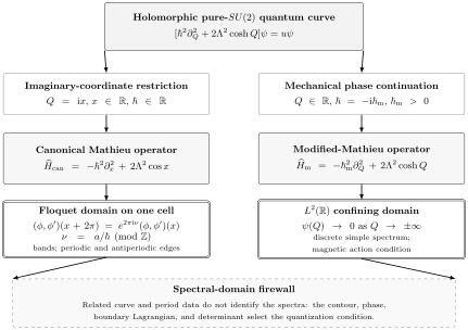
Two spectral realizations of one holomorphic differential family. The left lane fixes a Floquet multiplier on a compact cell and produces bands and band edges. The right lane phase-continues $\hbar=-\ii\hbar_{\mathrm m}$, imposes decay on the real line, and produces a discrete confining spectrum. Their curve and formal period data are related, but their domains select different Lagrangians and different exact quantization conditions.

The two lanes are analytically related, but they are not interchangeable by replacing $\cos$ with $\cosh$ in a final formula. The coordinate rotation changes the contour, the phase continuation rotates the WKB exponent and Borel ray, and the domain changes the global connection problem.

The first Floquet pole is resolved by a two-state problem

The Page 6 canonical Bloch ansatz gives the exact recurrence

$$\left[ (a+n\hbar)^2-u \right]c_n + \Lambda^2 \left( c_{n-1}+c_{n+1} \right) =0.$$

Away from $2a/\hbar\in\mathbb Z$, ordinary perturbation theory about $c_0=1$ yields

$$\begin{aligned} u(a,\hbar) ={}& a^2 + \frac{\Lambda^4}{a^2-(a-\hbar)^2} + \frac{\Lambda^4}{a^2-(a+\hbar)^2} +O(\Lambda^8) \\ ={}& a^2 + \frac{2\mathfrak q}{4a^2-\hbar^2} +O(\mathfrak q^2). \end{aligned}$$

The pole at $2a=\hbar$ occurs because the unperturbed modes $n=0$ and $n=-1$ have the same energy. Retain both before expanding. In the resonant scaling regime

$$\left|\frac{\Lambda^2}{\hbar^2}\right|\ll1, \qquad a-\frac{\hbar}{2} = O\!\left(\frac{\Lambda^2}{\hbar}\right),$$

eliminating the nonresonant modes gives the effective matrix

$$M_{\mathrm{res}} = \begin{pmatrix} a^2 & \Lambda^2 \\ \Lambda^2 & (a-\hbar)^2 \end{pmatrix} + O\!\left(\frac{\Lambda^4}{\hbar^2}\right).$$

Its two eigenvalues are

$$\begin{aligned} u_\pm ={}& \frac{ a^2+(a-\hbar)^2 }{2} \\ &\pm \sqrt{ \frac{\hbar^2(2a-\hbar)^2}{4} +\Lambda^4 } + O\!\left(\frac{\Lambda^4}{\hbar^2}\right). \end{aligned}$$

Exactly at the antiperiodic resonance,

$$a=\frac\hbar2, \qquad u_\pm = \frac{\hbar^2}{4} \pm\Lambda^2 +O\!\left(\frac{\Lambda^4}{\hbar^2}\right).$$

There is no divergent energy. The generic weak-coupling germ expanded one branch of the square root before approaching its branch point. The uniform local answer contains $\Lambda^2=\mathfrak q^{1/2}$, so it is not an integer-power instanton series about generic $a$.

Far enough from resonance, expanding the square root reproduces the $n=-1$ denominator; the nonresonant $n=+1$ state supplies the other denominator. Thus the same calculation both verifies the Page 6 coefficient and diagnoses its domain of validity.

What this resonance resolution does—and does not—show

The two-state calculation completes a singular weak-$\mathfrak q$ germ near one Floquet degeneracy. It does not Borel resum the small-$\hbar$ WKB series, impose $L^2(\mathbb R)$ decay, or construct a Fredholm determinant. Those are different completion problems.

Three independent axes of completion

The phrase “nonperturbative completion” is ambiguous unless its missing data are named. In this chapter at least three axes are independent.

Starting object	Expansion or locality	What it can miss	Typical completion
Generic Coulomb instanton germ	Integer powers of $\mathfrak q$ at fixed $(a,\hbar)$	Resonant mixing, fractional powers, other coupling charts, analytic continuation	Degenerate perturbation, a global characteristic equation, or continuation of the gauge germ
Formal quantum period	Even asymptotic powers of $\hbar$ at fixed curve data	Borel singularities, lateral ambiguity, terms $\ee^{-A/\hbar}$, Stokes jumps	Exact WKB, Borel–Écalle summation, Voros symbols, and a chamber prescription
Local NS or oper Lagrangian	Holomorphic data in one polarization	Boundary superpotential, real slice, Hilbert space, endpoint conditions, completeness	A second Lagrangian and a Wronskian, monodromy, or spectral determinant

The axes do not contain one another. For example, a convergent sum of all integer powers of $\mathfrak q$ may still have only a formal small-$\hbar$ expansion. Conversely, a Borel-resummed period at one fixed $\mathfrak q$ does not decide whether the wavefunction is periodic, antiperiodic, outgoing, or square-integrable.

For pure $SU(2)$, the finite-$\hbar$ instanton expansion is stronger than a formal WKB series. Where its weak-coupling $\Lambda$-series converges, it defines exact quantum periods as functions of $\hbar$; Grassi–Gu–Mariño describe a nonzero radius around the semiclassical region as expected. The result may still require analytic continuation beyond that domain, and exact periods are not yet a spectrum until the second Lagrangian, operator domain, quantization condition, and Matone energy map have been fixed.

Gauge instantons are nonperturbative in the ultraviolet coupling

With

$$\mathfrak q = \mu^4 \ee^{2\pi\ii\tau_{\mathrm{UV}}(\mu)}$$

up to the strong-scale scheme, the term $\mathfrak q^k$ is nonperturbative in ordinary microscopic gauge perturbation theory. Equivalently, the dimensionless instanton factor is $\mathfrak q/\mu^4$. “All instantons” means that all such integer powers have been retained in the selected block. The coefficientwise generic-$a$ germ displays only integer powers and therefore does not by itself resolve the $\mathfrak q^{1/2}$ branch at resonance; resumming or reorganizing all relevant sectors can encode that branch. “All instantons” still says nothing by itself about $\ee^{-A/\hbar}$ sectors or a WKB summation prescription.

All-orders WKB is still only a formal sector

A formal period has the structure

$$\Pi_\gamma^{\mathrm{formal}} (u,\hbar) = \sum_{k\geq0} \Pi_{\gamma,k}(u)\hbar^{2k}.$$

Even knowing every coefficient does not specify a function. Along a regular Borel direction $\theta$, one may define a sum $\mathcal S_\theta\Pi_\gamma$; on a singular direction one must choose $\mathcal S_{\theta+}$ or $\mathcal S_{\theta-}$ and transform the associated Voros symbols by the chamber’s Stokes automorphism. Two analytic functions with the same formal series can differ by

$$\Delta\Pi_\gamma \sim \ee^{-A/\hbar}.$$

The phase continuation $\hbar=-\ii\hbar_{\mathrm m}$ rotates the exponential and the Borel ray. A prescription called “positive direction” before the continuation need not remain nonsingular afterward.

A resummed period is not yet a determinant

Closed periods are coordinates on monodromy or character varieties. A boundary determinant also knows how normalized solutions are attached to endpoints or Stokes sectors. Local connection factors, open actions, and Stokes matrices can contribute even when the relevant closed period has been resummed. This is why exponentially small band widths or connection amplitudes can be invisible to a bare all-orders Bohr–Sommerfeld equation.

Three objects called TBA

The NS limit-shape saddle, the exact-WKB/GMN integral equations for resummed periods, and a Zamolodchikov-type integral equation for a spectral determinant can all have a thermodynamic-Bethe-ansatz form. They have different unknowns, kernels, asymptotics, and outputs. Chapters 12–13 develop the functional-relation and integral-equation viewpoints; no equality among these constructions is inferred from the shared acronym.

Modified Mathieu shows how NS data can enter an exact determinant

The warning “NS is not automatically a spectrum” does not mean that NS data can never determine one. The confining $SU(2)$ benchmark is a case where, after every missing choice is supplied, a gauge-resummed NS free energy enters a closed Fredholm-determinant formula.

To avoid silently mixing the Page 6 crosswalk with a published spectral identity, this subsection temporarily uses the source variables of Grassi–Gu–Mariño:

$$\left( E_{\mathrm s}, a_{\mathrm s}, \hbar_{\mathrm s}, F_{\mathrm{NS}}^{\mathrm s} \right).$$

Relative to the book’s unshifted $SU(2)$ operator and the Page 6 cycle orientation,

$$E_{\mathrm s}=u, \qquad a_{\mathrm s}=2a, \qquad \hbar_{\mathrm s}=-\hbar_{\mathrm m}.$$

The sign of $\hbar_{\mathrm s}$ is harmless for the differential expression, which contains its square, but it matters in period and quantization formulas. The published determinant formula is stated on the positive real $\hbar_{\mathrm s}$ ray; the relation $\hbar_{\mathrm s}=-\hbar_{\mathrm m}$ is the book’s analytic phase-and-cycle continuation, not literally that source ray. Its period and NS data must be continued as part of the same package. The source exact periods are normalized by

$$\begin{aligned} \Pi_A^{\mathrm{ex}} &= 2\pi a_{\mathrm s}(E_{\mathrm s},\hbar_{\mathrm s}), \\ \Pi_B^{\mathrm{ex}} &= 2\ii \partial_{a_{\mathrm s}} F_{\mathrm{NS}}^{\mathrm s} \bigg|_{a_{\mathrm s}=a_{\mathrm s}(E_{\mathrm s},\hbar_{\mathrm s})}. \end{aligned}$$

Thus $a_{\mathrm s}$ is the quantum mirror map evaluated at the spectral energy, not an independent argument of the determinant.

The domain supplies an entire spectral function

Let $\widehat H_{\mathrm m}^{\mathrm s}$ denote the source’s positive modified-Mathieu operator on $L^2(\mathbb R)$. Its inverse is trace class, so

$$\Xi_{\mathrm s}(E_{\mathrm s}) = \det\!\left( 1-E_{\mathrm s} (\widehat H_{\mathrm m}^{\mathrm s})^{-1} \right) = \prod_{n\geq0} \left( 1-\frac{E_{\mathrm s}}{E_n} \right)$$

is entire and vanishes precisely at the $L^2$ eigenvalues. That entireness is an operator-theoretic fact. In the source convention, GGM derive the following model-specific representation through the TS/ST construction and test it against TBA and spectral traces:

$$\Xi_{\mathrm s}(E_{\mathrm s}) = A(\hbar_{\mathrm s}) \frac{ \displaystyle \cosh\!\left( \frac{\Pi_B^{\mathrm{ex}}}{2\hbar_{\mathrm s}} \right) }{ \displaystyle \sinh\!\left( \frac{\Pi_A^{\mathrm{ex}}}{2\hbar_{\mathrm s}} \right) },$$

where $A(\hbar_{\mathrm s})$ is independent of energy and is fixed, for example, by $\Xi_{\mathrm s}(0)=1$. Every symbol in this equation is part of one normalization package.

Where the denominator is finite, the zeros of the numerator give

$$\frac{\Pi_B^{\mathrm{ex}}}{2\hbar_{\mathrm s}} = \ii\pi \left( k+\frac12 \right), \qquad k\in\mathbb Z,$$

and hence

$$\partial_{a_{\mathrm s}} F_{\mathrm{NS}}^{\mathrm s} = \pi\hbar_{\mathrm s} \left( k+\frac12 \right).$$

This is the modified-Mathieu/Toda quantization condition in the stated source convention; a physical branch reindexes its levels by $n=0,1,2,\ldots$. At a simultaneous denominator zero, the completed ratio—not the numerator alone—decides whether a residual zero remains. The condition is not obtained by setting a random derivative of the Page 4 local block equal to the right-hand side. The $L^2$ boundary condition, mechanical phase, magnetic polarization, energy map, source normalization, analytic continuation of the weak gauge germ, and half-integer zero condition encoded by the determinant have all already been selected.

The book crosswalk exposes the half shift

The Page 6 period translation converts the source determinant into a compact house form. In the GGM-calibrated subtraction, cycle, and energy scheme,

$$\begin{aligned} \Pi_A^{\mathrm{book}} &= 2\pi\ii a, \\ \Pi_B^{\mathrm{book}} &= -\hbar \partial_a\mathcal W_{\mathrm{NS}}^{\mathrm{loc}}, \qquad \hbar=-\ii\hbar_{\mathrm m}. \end{aligned}$$

Absorbing the nonzero, energy-independent normalization into $C(\hbar_{\mathrm m},\Lambda)$ gives

$$\Xi_{\mathrm m}(u;\hbar_{\mathrm m}) = C(\hbar_{\mathrm m},\Lambda) \frac{ \displaystyle \cosh\!\left( \frac12 \partial_a\mathcal W_{\mathrm{NS}}^{\mathrm{loc}} \right) }{ \displaystyle \sinh\!\left( \frac{2\pi\ii a}{\hbar} \right) }.$$

The numerator zeros obey

$$\partial_a\mathcal W_{\mathrm{NS}}^{\mathrm{loc}} = (2n+1)\pi\ii,$$

so the local derivative has exponential $-1$, not $+1$. The universal vacuum equation can be represented in the Page 4 $\exp(+\partial\mathcal W)=1$ bookkeeping by an affine second-Lagrangian term:

$$\partial_a\mathcal W^\infty = \pi\ii \pmod{2\pi\ii} \quad\Longrightarrow\quad \exp\!\left( \partial_a\mathcal W_{\mathrm{eff}} \right) =1.$$

This is a bookkeeping realization of the determinant-selected half shift, not a derivation of a unique microscopic boundary superpotential from the Fredholm formula. It is not a logarithm-sheet change, because an allowed sheet change adds an even multiple of $\pi\ii$ to the derivative. Linear or quadratic changes of the local NS scheme must be transferred consistently into the chosen $\mathcal W^\infty$.

Entirety is a global pole-cancellation test

The displayed ratio appears to have poles when $\sinh(\Pi_A^{\mathrm{ex}}/(2\hbar_{\mathrm s}))=0$. The true Fredholm determinant cannot have them: it is entire in $E_{\mathrm s}$. The analytic continuation of the numerator and the period data must cancel every would-be singularity. This is a stronger check than verifying a few weak-coupling coefficients or solving only the numerator equation.

In house variables the denominator divisor is

$$\sinh\!\left( \frac{2\pi\ii a}{\hbar} \right)=0 \quad\Longleftrightarrow\quad \frac{2a}{\hbar}\in\mathbb Z.$$

Under the analytic source-to-book crosswalk, this is the continuation of the same algebraic locus that produces canonical-Floquet resonances. It is not the same physical spectral problem. In the canonical lane, coefficient poles reorganize into branch cuts and band-edge splittings; in the confining lane, the completed $L^2$ Fredholm determinant is entire and its apparent divisor cancels. That global cancellation need not occur coefficient by coefficient in $\mathfrak q$.

The same lesson applies to Gamma-function and instanton denominators. A pole in one chart can be a necessary intermediate feature of a globally regular determinant. Declaring that pole a spectral level before assembling the full function reverses the logic.

In GGM’s original positive-$\hbar_{\mathrm s}$ sector, a negative-energy representation of this determinant separates two saddle contributions, the second exponentially small as $\hbar_{\mathrm s}\to0^+$. Under phase continuation the dominant and subdominant saddles can exchange. This is a concrete spectral contribution beyond a bare formal small-$\hbar$ sector, and it is logically distinct from the $\mathfrak q^{1/2}$ Floquet resonance resolution.

Special success, not automatic universality

For the two-particle periodic Toda system, the NS and modified-Mathieu $L^2$ spectral problems coincide after the stated choices, and the quantization condition has a direct derivation from the Toda Baxter equation. In higher-rank or different geometric-engineering problems, an NS Bethe problem and another proposed spectral realization can be different. The $SU(2)$ determinant is a calibration example, not a license to omit the spectral passport elsewhere.

The harmonic bottom checks the half shift

Near the minimum $Q=0$,

$$2\Lambda^2\cosh Q = 2\Lambda^2 +\Lambda^2Q^2 +O(Q^4).$$

Here and below choose $\Lambda=\sqrt{\Lambda^2}>0$ on the real mechanical slice. The book’s mechanical operator then has the leading spectrum

$$u_n = 2\Lambda^2 +(2n+1)\Lambda\hbar_{\mathrm m} +O(\hbar_{\mathrm m}^2), \qquad n=0,1,2,\ldots.$$

The zero-point term is the elementary local check behind the half-integer in the magnetic action condition. It does not prove the global determinant formula, but any proposed translation that loses this term has the wrong phase, cycle, or boundary convention.

A completed comparison proceeds through zero sets

For a new gauge/ODE pair, the safest comparison is not a slogan about “exact NS quantization” but a sequence of independently testable maps.

1. Construct the local NS datum. Fix $Z_{\mathrm{Nek}}$, the connected limit, subtraction, mass convention, and coupling chart.
2. Declare what is dynamical. Identify the twisted-chiral variables, integral flux lattice, global gauge quotient, and any constraints.
3. Add the second Lagrangian. State $\mathcal W^\infty$, twists, theta angles, and the polarization in which the vacuum equation is written.
4. Solve branch-invariantly. Use the exponentiated equation first; choose a lift only for calculation and track sheet changes.
5. Fix the quantum-curve passport. Supply the operator, ordering, half-form, mass and energy shifts, and the quantum mirror map.
6. Choose the analytic realization. Give the contour, real or complex slice, Hilbert space, domain, endpoint or Floquet data, and Stokes sectors.
7. Complete the periods. State whether they are formal, convergent in $\mathfrak q$, Borel summed in $\hbar$, lateral, or defined by an integral equation.
8. Construct the spectral function. Use a normalized Wronskian, Evans/Jost function, monodromy discriminant, or Fredholm determinant.
9. Compare zero sets. Check the candidate Bethe values against the spectral zeros with multiplicity, including resonances and limiting cases.
10. Test completeness. Exclude spurious roots, missing parity or Weyl sectors, and roots outside the declared domain.

Four checks are especially efficient:

• recover the classical action lattice as $\hbar\to0$;
• reproduce a local harmonic, free, or hypergeometric limit;
• verify weak-coupling coefficients away from resonance and use a uniform treatment at resonance;
• compare a boundary determinant or high-precision shooting spectrum, not merely one period series.

What Chapter 10 has established

The chapter now supplies a complete chain of conditional objects:

$$\begin{gathered} \text{four-dimensional theory and Coulomb geometry} \\ \Downarrow \\ (\Sigma,\lambda_{\mathrm{SW}},A,B) \longrightarrow Z_{\mathrm{Nek}} \longrightarrow \mathcal W_{\mathrm{NS}}^{\mathrm{loc}}, \\ \Downarrow\quad \text{operator, ordering, cycles, and normalization} \\ \text{quantum curve and conditional WKB–NS periods}, \\ \Downarrow\quad \text{Matone/accessory and boundary Lagrangian data} \\ \text{off-shell Hamiltonian coordinates and Bethe-vacuum candidates}, \\ \Downarrow\quad \text{domain, Stokes data, and spectral completion} \\ \text{a model-specific exact spectrum}. \end{gathered}$$

Only the arrows whose hypotheses have been supplied may be used. The NS partition function determines powerful holomorphic period and Yang–Yang data. It does not universally choose an operator ordering, wavefunction, real slice, boundary condition, Borel sum, or complete spectrum.

Chapter 11 adds the AGT bridge. It will distinguish the nondegenerate four-point block that represents a gauge partition function from the extra degenerate insertion whose BPZ equation supplies a wavefunction, and it will rebuild the ODE/CFT/gauge normalization dictionary without weakening the firewalls established here.

Interpretation and limitations

The exponentiated Bethe equation is exact as a low-energy vacuum condition in its declared effective theory. Its interpretation as a complete Bethe ansatz can additionally require a completeness theorem, control of singular roots, and a specified Hilbert space. Those are model-dependent analytic statements.

The two-state resonance calculation is deliberately modest. It proves that the first $2a=\hbar$ pole of the generic Floquet germ is removed by degenerate mixing and predicts the leading antiperiodic splitting. It does not prove the all-resonance characteristic-value theory, though it matches the standard Mathieu mechanism.

The modified-Mathieu determinant formula is quoted in its source normalization because partial translation is more dangerous than foreign notation. Page 6 gives the complete cycle and parameter crosswalk. A different energy shift, $2\pi$ normalization, cycle orientation, or sign of the mechanical continuation changes the printed formula.

Finally, “nonperturbative in $\mathfrak q$,” “beyond all orders in $\hbar$,” and “globally completed boundary problem” are not synonyms. The page’s central result is the dependency structure connecting them, not a universal closed quantization formula for every quantum Seiberg–Witten curve.

Common pitfalls

Extremizing a parameter. The Coulomb labels in a local $\mathbb C^2$ block are fixed boundary data. State the mechanism that makes them dynamical and add its boundary contribution before imposing a vacuum equation.

Treating a lift as invariant. The equation $\partial_a\mathcal W=2\pi\ii n$ changes under a logarithm-sheet shift. The exponential equation is invariant; the printed integer must move with the sheet.

Using the wrong constrained derivative. On an $SU(N)$ slice, vary independent traceless coordinates or subtract the eigenvalue equations. A single unconstrained $U(N)$ derivative carries the center-of-mass direction.

Calling every Bethe root an eigenvalue. First map the root to the operator coefficient, then test the declared boundary determinant. Domain, parity, Weyl, and completeness information cannot be inferred from the critical equation alone.

Identifying canonical and modified Mathieu. The substitutions $Q=\ii x$ and $\hbar=-\ii\hbar_{\mathrm m}$ lead to different contours and domains. One fixes a Floquet multiplier; the other imposes decay on the real line.

Reading equivariant poles as levels. At $2a=\hbar$, ordinary perturbation divided by a vanishing energy difference. Diagonalize the resonant subspace; the two characteristic values are finite and split by $2\Lambda^2+O(\Lambda^4/\hbar^2)$.

Using “all instantons” as “exact in every sense.” It specifies the $\mathfrak q$ expansion of one gauge block. It does not choose a Borel sum in $\hbar$, a Stokes chamber, or a boundary determinant.

Copying the modified-Mathieu NS condition alone. Its half shift, phase, magnetic polarization, and normalization belong to the $L^2$ determinant package. Importing only the final derivative equation can change the spectral problem.

Exercises

1. Check branch invariance

Let

$$\mathcal W'(a) = \mathcal W(a)+2\pi\ii k a+c, \qquad k\in\mathbb Z.$$

Show that the exponentiated vacuum equation is unchanged and determine how the lifted integer transforms.

Solution

Differentiation gives

$$\partial_a\mathcal W' = \partial_a\mathcal W+2\pi\ii k.$$

Hence

$$\exp(\partial_a\mathcal W') = \exp(\partial_a\mathcal W).$$

If $\partial_a\mathcal W=2\pi\ii n$ on the old sheet, then $\partial_a\mathcal W'=2\pi\ii(n+k)$. The same vacuum is labeled by $n'=n+k$.

2. Add an affine boundary term

Take

$$\mathcal W^\infty(a) = 2\pi\ii\xi a, \qquad \xi\in\mathbb C.$$

Write the lifted vacuum equation for $\mathcal W_{\mathrm{eff}}=\mathcal W_{\mathrm{NS}}^{\mathrm{loc}}+ \mathcal W^\infty$. Explain why a nonintegral $\xi$ is boundary data, not a relabeling of the flux lattice.

Solution

The equation is

$$\partial_a\mathcal W_{\mathrm{NS}}^{\mathrm{loc}} +2\pi\ii\xi = 2\pi\ii n,$$

or

$$\partial_a\mathcal W_{\mathrm{NS}}^{\mathrm{loc}} = 2\pi\ii(n-\xi).$$

An integral $\xi$ can be absorbed into $n$. A nonintegral $\xi$ shifts the boundary Lagrangian relative to the integral lattice and cannot be removed by an allowed sheet relabeling.

3. Remove the SU(2) center-of-mass direction

For a function $\mathcal W(a_1,a_2)$ restricted by $a_1+a_2=0$, set $a_1=a$ and $a_2=-a$. Derive the tangent derivative and show that only the difference of two lifted $U(2)$ equations is independent.

Solution

The chain rule gives

$$\frac{\dd}{\dd a}\mathcal W(a,-a) = \partial_{a_1}\mathcal W - \partial_{a_2}\mathcal W.$$

Writing $\partial_{a_\alpha}\mathcal W=2\pi\ii n_\alpha+\lambda$ and subtracting eliminates the multiplier:

$$\frac{\dd}{\dd a}\mathcal W(a,-a) = 2\pi\ii(n_1-n_2).$$

The sum points normal to the traceless slice and is not a second $SU(2)$ equation.

4. Continue a transverse Bethe root

Let

$$F_i(\boldsymbol a,s) = \partial_{a^i}\mathcal W_{\mathrm{eff}} -2\pi\ii n_i$$

depend on a parameter $s$. Assuming the Hessian $\mathcal H$ is invertible, derive $\dd a^i/\dd s$ along the vacuum branch.

Solution

Differentiate $F_i(\boldsymbol a(s),s)=0$:

$$\mathcal H_{ij} \frac{\dd a^j}{\dd s} + \partial_s\partial_{a^i} \mathcal W_{\mathrm{eff}} =0.$$

Therefore

$$\frac{\dd a^i}{\dd s} = - (\mathcal H^{-1})^{ij} \partial_s\partial_{a^j} \mathcal W_{\mathrm{eff}}.$$

Invertibility is exactly the local transversality condition.

5. Derive both Mathieu restrictions

Starting from

$$\left[ \hbar^2\partial_Q^2 +2\Lambda^2\cosh Q \right]\psi=u\psi,$$

derive the canonical Mathieu operator using $Q=\ii x$ and the modified operator using $\hbar=-\ii\hbar_{\mathrm m}$. State the boundary data that distinguish them.

Solution

For $Q=\ii x$, $\partial_Q^2=-\partial_x^2$ and $\cosh Q=\cos x$, so

$$\left[ -\hbar^2\partial_x^2 +2\Lambda^2\cos x \right]\phi=u\phi.$$

It is posed on a compact cell with quasi-periodic values of both $\phi$ and $\phi'$. For real $Q$ and $\hbar=-\ii\hbar_{\mathrm m}$,

$$\left[ -\hbar_{\mathrm m}^2\partial_Q^2 +2\Lambda^2\cosh Q \right]\psi=u\psi.$$

It is posed on the real line with $L^2$ decay at both ends. The differential family is related; the domains are not.

6. Recover the one-instanton Floquet coefficient

Use second-order perturbation theory for the mode $n=0$ in the Page 6 recurrence. Include the neighboring modes $n=\pm1$ and show that the energy shift equals $2\mathfrak q/(4a^2-\hbar^2)$.

Solution

The potential couples neighboring Fourier modes with matrix element $\Lambda^2$. Thus

$$\begin{aligned} \Delta u^{(2)} &= \frac{\Lambda^4}{a^2-(a-\hbar)^2} + \frac{\Lambda^4}{a^2-(a+\hbar)^2} \\ &= \frac{\Lambda^4}{\hbar(2a-\hbar)} - \frac{\Lambda^4}{\hbar(2a+\hbar)} \\ &= \frac{2\Lambda^4}{4a^2-\hbar^2} = \frac{2\mathfrak q}{4a^2-\hbar^2}. \end{aligned}$$

The displayed denominators exclude $2a/\hbar=\pm1$. More generally, nondegenerate perturbation theory about the $n=0$ seed fails at every distinct degeneracy

$$\frac{2a}{\hbar}=-m, \qquad m\in\mathbb Z\setminus\{0\}.$$

Resonances with $|m|>1$ first enter through higher-order mixing. The case $m=0$ is the seed mode itself, not a distinct free-mode degeneracy.

7. Resolve the first resonance

Diagonalize

$$\begin{pmatrix} a^2 & \Lambda^2 \\ \Lambda^2 & (a-\hbar)^2 \end{pmatrix}$$

and evaluate the result at $a=\hbar/2$. What feature cannot appear in an integer-power series in $\mathfrak q=\Lambda^4$?

Solution

The eigenvalues of this truncated block are

$$u_\pm = \frac{a^2+(a-\hbar)^2}{2} \pm \sqrt{ \frac{\hbar^2(2a-\hbar)^2}{4} +\Lambda^4 } +O\!\left(\frac{\Lambda^4}{\hbar^2}\right).$$

At resonance,

$$u_\pm = \frac{\hbar^2}{4} \pm\Lambda^2 +O\!\left(\frac{\Lambda^4}{\hbar^2}\right).$$

The splitting is proportional to $\Lambda^2=\mathfrak q^{1/2}$, which is invisible to a generic integer-power instanton germ.

8. Check the modified-Mathieu zero-point term

Expand the real-cosh potential near its minimum and compute the leading small-$\hbar_{\mathrm m}$ spectrum.

Solution

Choose $\Lambda=\sqrt{\Lambda^2}>0$ on the mechanical slice. Since

$$2\Lambda^2\cosh Q = 2\Lambda^2+\Lambda^2Q^2+O(Q^4),$$

the leading operator above the minimum is

$$-\hbar_{\mathrm m}^2\partial_Q^2 +\Lambda^2Q^2.$$

Its eigenvalues are $(2n+1)\Lambda\hbar_{\mathrm m}$. Hence

$$u_n = 2\Lambda^2 +(2n+1)\Lambda\hbar_{\mathrm m} +O(\hbar_{\mathrm m}^2).$$

9. Read the determinant zero correctly

In the source convention, assume

$$\Xi_{\mathrm s} = A \frac{ \cosh(\Pi_B^{\mathrm{ex}}/(2\hbar_{\mathrm s})) }{ \sinh(\Pi_A^{\mathrm{ex}}/(2\hbar_{\mathrm s})) }, \qquad \Pi_B^{\mathrm{ex}} =2\ii\partial_{a_{\mathrm s}}F_{\mathrm{NS}}^{\mathrm s}.$$

Derive its numerator quantization condition. Why does a zero of the denominator alone not define an eigenvalue?

Solution

The zeros of $\cosh z$ are $z=\ii\pi(n+1/2)$. Therefore

$$\partial_{a_{\mathrm s}}F_{\mathrm{NS}}^{\mathrm s} = \pi\hbar_{\mathrm s} \left(n+\frac12\right), \qquad n\in\mathbb Z.$$

A denominator zero is a putative pole, not by itself a zero of $\Xi_{\mathrm s}$. Because a Fredholm determinant is entire, the analytically continued numerator and period data must cancel the singularity. After that cancellation, a coincident eigenvalue would still require a residual zero of the completed entire function.

10. Name the missing completion

For each term or datum, name the completion layer to which it belongs and state any condition needed before it becomes ODE spectral data:

$$\mathfrak q^{1/2}, \qquad \ee^{-A/\hbar}, \qquad \mathcal W^\infty, \qquad D(E)=W[\psi_{\mathrm L},\psi_{\mathrm R}].$$

Solution

• $\mathfrak q^{1/2}$ reorganizes the weak-coupling expansion near a resonance.
• $\ee^{-A/\hbar}$ is beyond all orders in the formal WKB expansion.
• $\mathcal W^\infty$ supplies the second, boundary Lagrangian needed for the vacuum problem.
• $D(E)$ completes the global boundary-value problem and defines its spectral zero set.

$\mathcal W^\infty$ is boundary-Lagrangian data for the vacuum problem. It becomes spectral data only after a separate dictionary identifies that Lagrangian with the declared ODE boundary condition. The determinant $D(E)$ belongs to the ODE side and defines the spectral zero set; the two must be matched, not identified.

References

• N. A. Nekrasov and S. L. Shatashvili, “Quantization of Integrable Systems and Four Dimensional Gauge Theories”, in XVIth International Congress on Mathematical Physics (2010), 265–289. Section 2 derives the lifted and exponentiated vacuum equations from the two-dimensional effective potential. Section 5.1.3 distinguishes the $L^2$ periodic-Toda realization from the imaginary-periodic one and identifies, for two particles, modified versus canonical Mathieu; the later spectrum-of-observables subsection states the dual action-lattice conditions and Hamiltonian values in the source convention.
• N. A. Nekrasov and S. L. Shatashvili, “Supersymmetric Vacua and Bethe Ansatz”, Nuclear Physics B Proceedings Supplements 192–193 (2009), 91–112. Section 2.3 explains the flux sum, large-gauge shifts, and the single-valued exponentiated vacuum equation underlying the branch discussion; equations (2.33)–(2.34) give its lifted and invariant forms.
• N. A. Nekrasov, V. Pestun, and S. Shatashvili, “Quantum Geometry and Quiver Gauge Theories”, Communications in Mathematical Physics 357 (2018), 519–567. Sections 1.1.3–1.1.5 separate universal local and boundary contributions to the twisted superpotential. Their overall superpotential sign is opposite to the Page 4 house convention and must be translated as one package. Section 2.2, equations (2.23)–(2.25), treats $a$ as framing data at infinity; Section 3.3.1 emphasizes that the limit-shape roots build the superpotential at fixed $a$, before any Coulomb-vacuum equation is imposed.
• N. A. Nekrasov, A. Rosly, and S. Shatashvili, “Darboux Coordinates, Yang–Yang Functional, and Gauge Theory”, Nuclear Physics B Proceedings Supplements 216 (2011), 69–93. Equations (20)–(23) formulate the generating function in a chosen Darboux chart and show where the second Lagrangian enters. The broad correspondence is presented there as coordinate-dependent and conjectural.
• N. Nekrasov and E. Witten, “The Omega Deformation, Branes, Integrability, and Liouville Theory”, Journal of High Energy Physics 09 (2010) 092. Sections 2.1–2.2 distinguish formal holomorphic quantization from the real middle-dimensional cycle that supplies a Hilbert space. Section 3.4 explains how a far-end boundary condition selects a second Lagrangian and how transverse intersections produce states.
• A. Gorsky, K. Milekhin, and N. Sopenko, “Bands and Gaps in Nekrasov Partition Function”, Journal of High Energy Physics 01 (2018) 133. Section 2 separates the modified-Mathieu $L^2$ and canonical-Mathieu Bloch boundary conditions. Section 3.1 proposes and tests, in equations (26) and (30)–(38), a model-specific reorganization of poles at integral Floquet exponent into square-root cuts and split band edges. This supports the independently checked two-state resolution for the periodic, canonical problem without identifying it with the $L^2$ spectrum.
• K. K. Kozlowski and J. Teschner, “TBA for the Toda Chain”. The Baxter/TBA analysis in Sections 3.2–3.4 and Appendix C.3 derives the Nekrasov–Shatashvili Toda quantization conditions under stated analytic assumptions and relates them to a Yang-potential extremum. The remark following the theorem leaves global solvability, complex solutions, and uniqueness for a prescribed integer tuple open; this is model-specific analytic support, not a general completeness theorem.
• A. Grassi, J. Gu, and M. Mariño, “Non-Perturbative Approaches to the Quantum Seiberg–Witten Curve”, Journal of High Energy Physics 07 (2020) 106. Equations (4.12)–(4.18) develop the finite-$\hbar$ instanton series and source exact-period normalization; equations (4.37)–(4.40) continue beyond the direct weak-coupling series; and equations (4.50)–(4.54) compare WKB lateral sums and additional strong-coupling nonperturbative terms. Equations (5.6)–(5.7) give the modified-Mathieu Fredholm determinant, equation (5.16) its NS quantization condition, and the discussion after (5.27) the cancellation of would-be period and Gamma-function poles. Sections 3–4 separately compare Borel-resummed WKB periods with the gauge-resummed weak-coupling germ.
• A.-K. Kashani-Poor and J. Troost, “Pure N=2 Super Yang–Mills and Exact WKB”, Journal of High Energy Physics 08 (2015) 160. Section 3.3, especially equations (3.27)–(3.30), (3.47), and (3.50), computes quantum periods and shows that exact Floquet monodromy also contains Stokes-continuation data. Section 4’s transseries and worldsheet interpretation is conjectural, and the paper does not prove Borel summability of the proposed full transseries.
• G. Başar and G. V. Dunne, “Resurgence and the Nekrasov–Shatashvili Limit: Connecting Weak and Strong Coupling in the Mathieu and Lamé Systems”, Journal of High Energy Physics 02 (2015) 160. The all-orders Mathieu analysis relates perturbative and instanton sectors and makes explicit why exponentially small band and gap widths require more than a bare all-orders energy expansion.
• NIST Digital Library of Mathematical Functions, §28.2, Mathieu functions and §28.29, Hill’s equation and Floquet theory. These sections fix the standard Floquet terminology and the periodic, antiperiodic, parity, and characteristic-value structure used in the canonical lane.