Quantum Seiberg–Witten Curves and Ordering Data

Page 2 supplied a classical Seiberg–Witten curve, its distinguished differential, and an integral cycle lattice. Page 4 supplied a connected NS twisted superpotential. Neither datum is yet a quantum differential equation. Quantization begins only after choosing a Darboux chart, mapping the surviving equivariant parameter to a commutator, selecting a polarization and ordering prescription, and saying what the wavefunction represents.

The result is therefore a package, not an equation with hats added to its variables. Its first invariant check is modest but decisive: the principal symbol must recover the declared classical curve in the same coordinates and units. Subprincipal terms, mass shifts, half-density laws, and wavefunction normalizations then distinguish quantum curves with the same classical limit. This page constructs that package and tests it on pure $SU(2)$. It does not yet identify WKB periods with NS periods or turn the resulting operator into a complete spectral problem.

Page question

Which data turn a classical Seiberg–Witten curve into a reproducible quantum operator, and which apparent ambiguities are ordering, polarization, coordinate, or wavefunction choices rather than new classical geometry?

Status ledger

Statement used on this page	Status
A quantum curve has the classical Seiberg–Witten curve as principal symbol	Defining semiclassical requirement in a declared Darboux chart
The classical equation uniquely fixes its quantization	False
$\hbar:=\epsilon_1$	The book’s holomorphic NS parameter; it is not silently identified with a real mechanical Planck constant
$\varkappa$	Canonical commutator parameter, with $[\widehat Q,\widehat P]=\varkappa$
Left, right, and Weyl orderings have the same principal symbol	Exact for the displayed polynomial example; their subprincipal terms differ
Conjugate differential expressions are automatically the same spectral problem	False unless the conjugation also transports the function space and domain
A scalar $SL(2)$ oper is a function-valued equation	Only locally; globally its wavefunction is a section of $K^{-1/2}$ after choosing a theta characteristic
The bulk $Z_{\mathrm{Nek}}$ is the oper wavefunction	False; it has no defect coordinate
A normalized surface-defect amplitude can obey a quantum-curve equation	Established in specified gauge-theory/defect constructions, not a theorem for every Seiberg–Witten geometry
The pure-$SU(2)$ benchmark gives a holomorphic quantum SW equation	Exact after the chart, ordering, and Page 2 normalization are declared
The real-cosh modified-Mathieu operator uses the same printed $\hbar=\epsilon_1$	False; it is the phase-continued mechanical convention $\hbar=-\ii\hbar_{\mathrm m}$
The displayed pure-$SU(2)$ eigenvalue is $u$	Declared minimal operator convention in the Page 2 normalization; the principal symbol still permits $E_{\mathrm{op}}=u+O(\hbar)$
Differential and difference polarizations are spectrally equivalent	Formal at the Heisenberg-algebra level; analytic equivalence needs an integral kernel, contours, and domains
The operator alone fixes normalized quantum periods or a spectrum	False; Pages 6–8 add the missing data

Convention ledger

Datum	Convention on this page
Classical chart	Local Darboux coordinates $(Q,P)$ with canonical one-form $P\,\dd Q$
Seiberg–Witten normalization	$\lambda_{\mathrm{SW}}=c\,P\,\dd Q+\dd F$ with $c$ declared model by model
Canonical algebra	$[\widehat Q,\widehat P]=\varkappa$
Holomorphic NS lane	$\hbar:=\epsilon_1$, $\varkappa=-\hbar$, and $\widehat P=\hbar\partial_Q$
Mechanical lane	$\varkappa=\ii\hbar_{\mathrm m}$ and $\widehat P=-\ii\hbar_{\mathrm m}\partial_Q$
Phase crosswalk	The same operator is continued by $\hbar=-\ii\hbar_{\mathrm m}$
Dual polarization	$\widehat P=P$ and $\widehat Q=\varkappa\partial_P$
Ordering reference	Normal ordering means coefficient functions of $Q$ stand to the left of $\widehat P$; alternatives are written explicitly
Scalar oper	Acts on $K^{-1/2}$, with a chosen theta characteristic and puncture data
Mass label	The Page 3 equivariant label $\mu$ is held fixed unless a centered mass is named explicitly
Pure-$SU(2)$ logarithmic chart	$z=-\ee^Q$, so $\dd z/z=\dd Q$
Pure-$SU(2)$ energy	Unshifted benchmark $E_{\mathrm{op}}:=u$; finite quantum shifts remain separate data
Not fixed here	Quantum mirror map, period cycles, Borel chamber, accessory map, Hilbert space, boundary conditions, and nonperturbative completion

A quantum curve is a filtered operator package

Let a classical Seiberg–Witten curve be written locally as

$$H(Q,P;u,\boldsymbol m,\boldsymbol\Lambda)=0,$$

where $(Q,P)$ are Darboux coordinates. The symplectic form is $\dd P\wedge\dd Q$, while the distinguished one-form has the local shape

$$\lambda_{\mathrm{SW}} = c\,P\,\dd Q+\dd F.$$

The constant $c$ and the exact term are not decorative. The first fixes the units of periods; the second can change open integrals and endpoint normalizations even though it drops out of compact classical periods. A birational presentation that does not transport $\lambda_{\mathrm{SW}}$ has therefore not preserved the full classical datum.

To keep the phase convention visible, introduce a complex canonical parameter $\varkappa$ by

$$[\widehat Q,\widehat P]=\varkappa, \qquad \widehat P=-\varkappa\partial_Q.$$

This is notation for the quantization map, not a second physical deformation. The book’s physical NS variable remains $\hbar=\epsilon_1$; the holomorphic and mechanical identifications of $\varkappa$ are made explicitly below.

A local quantum curve is an equation

$$\widehat H_{\varkappa}\psi=0$$

for a filtered differential, difference, or more general pseudodifferential operator satisfying

$$\sigma_{\mathrm{pr}}(\widehat H_{\varkappa}) = H(Q,P;u,\boldsymbol m,\boldsymbol\Lambda).$$

Here the principal symbol is computed in the declared chart and commutator convention. For a normally ordered differential operator, one replaces

$$-\varkappa\partial_Q\longmapsto P$$

and retains the leading semiclassical term. If the printed operator has explicit $\varkappa$-dependent coefficients, only their leading terms enter the principal symbol; the rest are subprincipal or higher quantum data.

The definition is deliberately local. A global scalar equation also needs a line bundle, transition functions, and singularity data. A spectral operator needs still more: a real or complex slice, a function space, a domain, and boundary or Stokes conditions. Conflating those levels is the fastest route from a correct formal curve to an incorrect claim about eigenvalues.

The quantization passport

The following entries make a printed quantum curve reproducible.

Entry	Question it answers	What can change if it is omitted
Classical curve and differential	Which $H=0$ and which $\lambda_{\mathrm{SW}}$ are being quantized?	Energy and period normalizations
Darboux chart	Which variables obey the canonical bracket?	The expression of the symbol and allowed canonical transforms
Commutator map	Which deformation parameter equals $\varkappa$, with what sign or phase?	Every quantum correction and WKB phase
Polarization	Which variable multiplies and which differentiates or shifts?	Differential versus difference realization
Quantization map	Is the prescription normal, anti-normal, Weyl, or model-specific?	Subprincipal and higher symbols
Wavefunction bundle	Is $\psi$ a function, density, half-density, or section with monodromy?	Coordinate covariance and global signs
Observable	Which defect, brane, conformal block, or kernel produces $\psi$?	The equation and its normalization
Quantum parameter map	Are masses centered, and is the operator energy $u$ or a shifted modulus?	Local exponents and accessory terms
Analytic realization	Which contour, domain, and boundary/Stokes data are imposed?	The spectrum; deferred to Page 8

The last row is intentionally separated from formal quantization. It is possible to define and manipulate a quantum curve without choosing a Hilbert-space spectrum. It is not possible to quote the spectrum of that curve without doing so.

Same symbol does not mean same quantum curve

Two operators can have identical principal symbol and different subprincipal symbols. They can then have different local exponents, monodromy, quantum periods, or spectral determinants. Agreement as $\varkappa\to0$ is a necessary classical check, not an exact equivalence proof.

Ordering appears one level below the classical curve

Use the $Q$-polarization

$$\widehat P=-\varkappa\partial_Q, \qquad [\widehat Q,\widehat P]=\varkappa.$$

For a nonconstant coefficient $f(Q)$, the commutator is

$$\widehat P f = f\widehat P-\varkappa f'.$$

Consequently the three natural quantizations of the same classical monomial $f(Q)P$ are

$$\begin{aligned} \operatorname{Op}_{\mathrm L}(fP) &=f\widehat P, \\ \operatorname{Op}_{\mathrm R}(fP) &=\widehat P f =f\widehat P-\varkappa f', \\ \operatorname{Op}_{\mathrm W}(fP) &=\frac12 \left( f\widehat P+\widehat P f \right) =f\widehat P-\frac{\varkappa}{2}f'. \end{aligned}$$

All three have principal symbol $fP$. Their order-$\varkappa$ terms differ. More generally,

$$\operatorname{Op}_s(fP) = (1-s)f\widehat P+s\widehat P f = f\widehat P-s\varkappa f',$$

with $s=0,1/2,1$ giving left, Weyl, and right ordering. The parameter $s$ is not visible in the classical curve.

This elementary identity contains the general lesson. Replacing every $P$ by $-\varkappa\partial_Q$ is an ordering prescription only when all coefficient functions have already been placed on a declared side. For higher monomials, Weyl ordering symmetrizes over all positions; for matrix, difference, or elliptic operators, the relevant quantization map must be stated rather than guessed from typography.

Conjugation changes the printed subprincipal terms

Let $g(Q)$ be independent of negative powers of $\varkappa$ and define

$$\widehat H^{(g)} = \ee^{-g}\widehat H\ee^g.$$

Then

$$\ee^{-g}\widehat P\ee^g = \widehat P-\varkappa g'.$$

Thus conjugation leaves the principal symbol unchanged but alters the subprincipal operator. For a quadratic normal form,

$$\begin{aligned} &\ee^{-g} \left( \varkappa^2\partial_Q^2+V \right) \ee^g \\ &\quad= \varkappa^2\partial_Q^2 +2\varkappa^2g'\partial_Q +V +\varkappa^2 \left( g''+(g')^2 \right). \end{aligned}$$

If $\widehat H\psi=0$, then $\widehat H^{(g)}(\ee^{-g}\psi)=0$. This is an exact local change of wavefunction normalization. It becomes an equivalence of spectral operators only when multiplication by $\ee^{-g}$ is an invertible map between the chosen spaces and transports the domains and boundary conditions. A factor that grows at an endpoint can fail that test.

Not every ordering ambiguity is a conjugation. Conjugation preserves operator invariants within its analytic domain, whereas independent $\varkappa$-dependent potentials can change monodromy or spectrum. One must exhibit the intertwiner rather than infer it from a common principal symbol.

Half-density covariance fixes a quantum correction

Ordering is also affected by coordinate changes. Consider a scalar normal-form equation in a local coordinate $z$,

$$\left[ \varkappa^2\partial_z^2+V(z;\varkappa)-E \right] \psi(z)=0.$$

Let $z=z(w)$ be locally biholomorphic and set

$$s(w)=\frac{\dd z}{\dd w}.$$

Composing $\psi$ with $z(w)$ as though it were a scalar function introduces a first derivative. Normal form is preserved by the half-density transformation

$$\widetilde\psi(w) = s(w)^{-1/2}\psi(z(w)).$$

The combined potential transforms as

$$\begin{aligned} \widetilde{V-E}(w;\varkappa) &= s(w)^2 \left[ V(z(w);\varkappa)-E \right] \\ &\quad+ \frac{\varkappa^2}{2} \{z,w\}, \end{aligned}$$

where

$$\{z,w\} = \frac{z'''}{z'} -\frac32 \left( \frac{z''}{z'} \right)^2$$

is the Schwarzian derivative. The first term is the classical quadratic-differential transformation law. The Schwarzian is an order-$\varkappa^2$ correction forced by coordinate covariance; dropping it produces a different quantum equation.

On the mechanical lane $\varkappa=\ii\hbar_{\mathrm m}$, the leading term is $-\hbar_{\mathrm m}^2\partial_z^2$ and the Schwarzian contribution is $-\hbar_{\mathrm m}^2\{z,w\}/2$. Thus the unified formula carries the phase convention rather than hiding it in the potential.

The transformation law means that the wavefunction of a second-order $SL(2)$ oper is locally a section of $K^{-1/2}$, not an ordinary function. Globally one chooses a theta characteristic $K^{1/2}$, along with compatible puncture and monodromy data. The projective connection exists before that lift is chosen, but a particular scalar half-density equation does not. The construction and cocycle check were derived on Liouville Normal Form and SL(2) Opers.

An exponential-coordinate unit test

Take $V-E=0$ and $z=\ee^w$. Since

$$\{\ee^w,w\}=-\frac12,$$

the transformed equation is

$$\left[ \varkappa^2\partial_w^2 -\frac{\varkappa^2}{4} \right] \widetilde\psi=0.$$

The original solutions $1$ and $z$ become $\ee^{-w/2}$ and $\ee^{w/2}$, which solve the transformed equation. Without the Schwarzian term they would not. This exact two-solution check distinguishes a covariance correction from an optional semiclassical refinement.

Coordinate changes can mix several ledgers

A canonical change of phase-space coordinates transports $P\,\dd Q$; a change of the scalar ODE coordinate transports a half-density and its projective connection; a gauge transformation conjugates the operator. These operations can be combined in examples, but they are not synonyms and need not produce the same endpoint or monodromy normalization.

The gauge-theory wavefunction needs an observable

The bulk Nekrasov function depends on Coulomb parameters, masses, couplings, and equivariant weights. It has no ODE coordinate $z$. Consequently neither $Z_{\mathrm{Nek}}$ nor $\mathcal W_{\mathrm{NS}}^{\mathrm{loc}}$ is, by itself, a scalar wavefunction on the Seiberg–Witten curve.

In a class of surface-defect constructions, one instead has a defect partition function with an additional position or monodromy variable,

$$Z_{\mathrm{def}} = Z_{\mathrm{def}} (a,z;\epsilon_1,\epsilon_2).$$

After fixing the defect scheme and removing explicit normalization prefactors, its NS asymptotic can take the schematic form

$$\begin{aligned} Z_{\mathrm{def}} \left( a,z;\hbar,\epsilon_2 \right) &= \exp\!\left[ \frac{ \mathcal W_{\mathrm{bulk}}^{\mathrm{def}}(a;\hbar) }{\epsilon_2} \right] \\ &\quad\times \left[ \chi(a,z;\hbar)+O(\epsilon_2) \right]. \end{aligned}$$

Equivalently, the normalized defect amplitude is

$$\chi(a,z;\hbar) = \lim_{\epsilon_2\to0} \exp\!\left[ -\frac{ \mathcal W_{\mathrm{bulk}}^{\mathrm{def}}(a;\hbar) }{\epsilon_2} \right] Z_{\mathrm{def}}.$$

Here $\mathcal W_{\mathrm{bulk}}^{\mathrm{def}}$ denotes the common bulk exponent in the defect’s normalization. Before it is replaced by Page 4’s $\mathcal W_{\mathrm{NS}}^{\mathrm{loc}}$, any omitted one-loop term, counterterm, or $z$-independent prefactor must be translated explicitly. A coupling derivative can be insensitive to a coupling-independent omission even when the full generating function is not.

In the constructions where defect Ward identities close, this normalized object obeys an oper equation

$$\widehat H_z \left( u,\boldsymbol m,\boldsymbol\Lambda;\hbar \right) \chi(a,z;\hbar)=0.$$

The division of labor is important. The defect supplies the variable and wavefunction; the translated bulk NS function can supply coefficient data, often through a coupling derivative; and the Ward identity supplies the operator equation. A prefactor $\chi\mapsto F(z)\chi$ conjugates the printed operator. It may also shift local exponents if $F$ is multivalued. The defect type and normalization therefore belong in the quantization passport.

This mechanism is exact in the gauge-theory classes where it has been derived, including the surface-defect/oper constructions discussed in the references. It is not a universal recipe assigning a preferred wavefunction to every abstract Seiberg–Witten curve. Chapter 11 will separate the nondegenerate AGT block from the additional degenerate insertion that produces the BPZ/oper equation.

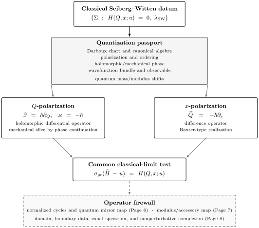
The classical pair $(\Sigma,\lambda_{\mathrm{SW}})$ does not choose an operator. A quantization passport fixes the Darboux chart, commutator map, polarization, ordering and subprincipal terms, wavefunction bundle and observable, and quantum parameter shifts. Different polarizations can realize the same principal symbol, but neither realization alone fixes normalized periods, the accessory map, or a spectral domain.

Pure SU(2): holomorphic quantization and modified Mathieu

Return to the normalization fixed on Page 2:

$$\Lambda^2 \left( z+\frac1z \right) = x^2-u, \qquad \lambda_{\mathrm{SW}} = \frac{1}{2\pi\ii} x\frac{\dd z}{z}.$$

Choose the logarithmic coordinate

$$z=-\ee^Q, \qquad \frac{\dd z}{z}=\dd Q.$$

The minus sign selects the positive-cosh presentation. It does not by itself select a real slice; reality of $Q$, $\Lambda$, and the operator parameter, together with a domain, is additional analytic data. The curve and differential become

$$\begin{aligned} H(Q,x;u) &:= x^2+2\Lambda^2\cosh Q-u=0, \\ \lambda_{\mathrm{SW}} &= \frac{1}{2\pi\ii}x\,\dd Q. \end{aligned}$$

Thus $x\,\dd Q=2\pi\ii\lambda_{\mathrm{SW}}$. The Darboux one-form used for the commutator is not numerically identical to the normalized Seiberg–Witten differential; their factor $2\pi\ii$ must survive any later period comparison.

The dimensional ledger is

$$[Q]=0, \qquad [x]=[\varkappa]=[\hbar]=[\hbar_{\mathrm m}]=[\Lambda]=1, \qquad [u]=2.$$

The book’s bare parameter remains the holomorphic NS variable $\hbar=\epsilon_1$. Choose

$$\varkappa=-\hbar, \qquad [\widehat Q,\widehat x]=-\hbar, \qquad \widehat x=\hbar\partial_Q.$$

Because $x^2$ and $\cosh Q$ contain no mixed monomial, this particular presentation has no ordering ambiguity. Its $Q$-polarized quantum curve in the holomorphic NS convention is

$$\boxed{ \widehat H_{\mathrm{hol}} = \hbar^2\partial_Q^2 +2\Lambda^2\cosh Q, \qquad \widehat H_{\mathrm{hol}}\psi=u\psi. }$$

The box is used here because this operator is the chapter’s calibration formula. Replacing $\hbar\partial_Q$ by $x$ gives

$$\sigma_{\mathrm{pr}} \left( \widehat H_{\mathrm{hol}}-u \right) = x^2+2\Lambda^2\cosh Q-u = H.$$

Every term has mass dimension two. These two checks catch the most common sign, scale, and factor errors before any WKB expansion is attempted.

The mechanical Planck constant is phase-continued

The familiar real-cosh modified-Mathieu expression uses a mechanical Planck constant $\hbar_{\mathrm m}$:

$$\widehat H_{\mathrm m} = -\hbar_{\mathrm m}^2\partial_Q^2 +2\Lambda^2\cosh Q.$$

It is the same holomorphic family after

$$\hbar=-\ii\hbar_{\mathrm m}, \qquad \varkappa=\ii\hbar_{\mathrm m}.$$

Indeed $\widehat x=\hbar\partial_Q =-\ii\hbar_{\mathrm m}\partial_Q$ then becomes the standard mechanical momentum. For real positive $(\hbar_{\mathrm m},\Lambda)$ and $Q\in\mathbb R$, the expression $\widehat H_{\mathrm m}$ admits the usual self-adjoint realization after a domain is chosen. That reality condition is a phase-continued slice of the holomorphic NS problem, not the identity $\hbar_{\mathrm m}=\epsilon_1$.

This crosswalk matters already in perturbation theory:

$$4a^2-\hbar^2 \quad\longmapsto\quad 4a^2+\hbar_{\mathrm m}^2.$$

The left denominator is the Page 4 holomorphic NS convention; the right is its value on the mechanical slice. Comparing them at the same printed real parameter would create a spurious sign disagreement.

Why some sources print E = 2u

Modified Mathieu is often written as

$$\left[ -\hbar_{\mathrm m}^2\partial_Q^2 +2\Lambda^2\cosh Q \right] \psi=E\psi.$$

For the unshifted benchmark declared here, $E_{\mathrm{op}}:=u$. This preserves the Page 2 classical normalization, but Page 2 alone does not exclude a finite correction $E_{\mathrm{op}}=u+O(\hbar)$. A source using $E=2u_{\mathrm{src}}$ has $u_{\mathrm{src}}=u/2$ relative to this unshifted benchmark. Importing its printed energy formula while retaining our periods would mix two normalizations.

Starting instead from $z=\ee^Q$ gives

$$x^2-2\Lambda^2\cosh Q=u.$$

The shift $Q\mapsto Q+\pi\ii$ reverses the sign of $\cosh Q$ and returns the displayed positive-potential form. On a complex curve this is an analytic coordinate change. Calling $Q\in\mathbb R$ and imposing $L^2(\mathbb R)$ conditions is an additional real-slice and domain choice, and it applies to the mechanical continuation rather than the same-real-$\hbar$ NS equation. That spectral choice belongs to Page 8.

The first WKB check is a Riccati equation

Use the local ansatz

$$\psi(Q) = \exp\!\left[ -\frac{1}{\varkappa} \int^Q P(q;\varkappa)\,\dd q \right].$$

Substitution into the differential equation gives the exact Riccati equation

$$P^2-\varkappa P' = u-2\Lambda^2\cosh Q.$$

Writing $P=P_0+\varkappa P_1+\cdots$ yields

$$P_0^2 = u-2\Lambda^2\cosh Q = x^2.$$

The leading WKB one-form is therefore $P_0\,\dd Q=x\,\dd Q$ on a chosen sheet, exactly the unnormalized Darboux one-form of the classical curve. This is a principal-symbol check, not yet the claim

$$\oint P\,\dd Q \stackrel{?}{=} 2\pi\ii \times \text{a normalized quantum SW period}.$$

Page 6 will formulate this identification conditionally, after declaring quantum cycles, parity conventions, the quantum mirror map, and Borel continuation; none follows from the operator alone.

The dual polarization gives a difference equation

Represent $x$ by multiplication and choose

$$\widehat Q=\varkappa\partial_x, \qquad [\widehat Q,\widehat x]=\varkappa.$$

Exponentiating the derivative translates the argument:

$$\begin{aligned} \ee^{\widehat Q}\Psi(x) &=\Psi(x+\varkappa), \\ \ee^{-\widehat Q}\Psi(x) &=\Psi(x-\varkappa). \end{aligned}$$

On the holomorphic NS lane $\varkappa=-\hbar$, the same quantized Hamiltonian becomes

$$\boxed{ x^2\Psi(x) +\Lambda^2 \left[ \Psi(x+\hbar) +\Psi(x-\hbar) \right] = u\Psi(x). }$$

At the formal algebraic level this is a Baxter-type difference realization of the same curve. Replacing the shift operators by $\ee^{\pm Q}$ gives

$$x^2+\Lambda^2 \left( \ee^Q+\ee^{-Q} \right)-u = H(Q,x;u).$$

The differential and difference equations are two polarizations of the same Heisenberg algebra. A Fourier-type transform can relate them formally, but spectral equivalence requires a specified transform kernel, integration contour, growth class, and transported domain. On the mechanical lane the shifts are $x\mapsto x\pm\ii\hbar_{\mathrm m}$; on the holomorphic lane they are $x\mapsto x\pm\hbar$. Either realization needs a shift-invariant lattice or an analytic domain large enough to evaluate the translated arguments. None of those analytic facts follows from the commutator.

Why the benchmark is unusually clean

The pure-$SU(2)$ Hamiltonian is a sum of a function of $x$ and a function of $Q$. It therefore avoids mixed-monomial ordering ambiguities in both displayed polarizations. This is a virtue for a calibration example, not evidence that ordering is absent from general quantum Seiberg–Witten curves.

Quantum parameter shifts belong to the operator dictionary

On the holomorphic NS lane, a general second-order quantum curve may have normal form

$$\left[ \hbar^2\partial_z^2 +U_0(z;u,\boldsymbol m) +\hbar U_1(z;u,\boldsymbol m) +\hbar^2U_2(z;u,\boldsymbol m) +\cdots \right] \psi=0.$$

Only $U_0$ is fixed by the classical symbol. The higher coefficients can encode ordering, the half-density correction, a defect normalization, or finite shifts of masses and moduli. These sources of quantum terms should be recorded separately even when they combine into one printed potential.

Centered and equivariant masses are different coordinates

Page 3 fixed the relation

$$\widehat m = \mu-\frac{\epsilon_1+\epsilon_2}{2}.$$

If the equivariant label $\mu$ is held fixed in the NS limit, then

$$\widehat m_{\mathrm{NS}} = \mu-\frac{\hbar}{2}.$$

A potential printed in terms of $\widehat m$ therefore differs at finite $\hbar$ from one printed in terms of $\mu$. Replacing one symbol by the other without the half-shift can change local exponents and monodromy. Conversely, a term such as $m(m+\hbar)$ in a quantum Hamiltonian can be a centered-mass effect, not an arbitrary ordering mistake. The declared mass coordinate, not the letter $m$, determines the comparison.

The operator energy need not equal the printed modulus

The classical curve fixes a leading map $E_{\mathrm{cl}}(u,\boldsymbol m,\boldsymbol\Lambda)$. At finite $\hbar$, a model can instead require

$$\begin{aligned} E_{\mathrm{op}} &= E_{\mathrm{cl}} \left( u,\boldsymbol m,\boldsymbol\Lambda \right) \\ &\quad+ \hbar e_1 \left( u,\boldsymbol m,\boldsymbol\Lambda \right) \\ &\quad+ \hbar^2 e_2 \left( u,\boldsymbol m,\boldsymbol\Lambda \right) +\cdots. \end{aligned}$$

An $O(\hbar)$ or $O(\hbar^2)$ shift leaves the principal symbol unchanged. It is fixed by an independent normalization: for example a Ward identity, a quantum Matone relation, an accessory-parameter derivative, or a calibrated weak-coupling limit. Page 7 derives and tests such maps in stated model and convention packages. For the pure-$SU(2)$ benchmark on this page we have made the minimal operator convention $E_{\mathrm{op}}:=u$; this is a declared choice, not a theorem that all quantum modulus shifts vanish in every presentation.

The quantum mirror map is a separate relation between the operator modulus and a normalized quantum period,

$$a=a(u;\hbar), \qquad u=u(a;\hbar).$$

It is not determined by the principal symbol alone. Fixing it requires the cycle and period conventions of Page 6, while identifying the same $u$ with an accessory parameter requires Page 7.

A reproducible quantum-curve audit

For a proposed gauge/ODE dictionary, the following order minimizes hidden convention changes.

1. Freeze the classical passport. Write the exact curve, differential, mass coordinates, modulus, scale, and dimensions.
2. Choose a Darboux chart. Verify $\lambda_{\mathrm{SW}}=cP\,\dd Q+\dd F$ and record $c$.
3. Declare the canonical algebra. State $[\widehat Q,\widehat P]=\varkappa$ and map $\varkappa$ to the holomorphic or mechanical deformation parameter, including its sign or phase.
4. Name the quantization map. Give the polarization, ordering, and all explicit subprincipal terms.
5. Name the wavefunction. State its bundle, defect or observable, prefactor, and monodromy normalization.
6. Translate quantum parameters. Center masses explicitly and keep $E_{\mathrm{op}}$, $u$, and accessory parameters distinct until a relation is derived.
7. Run local checks. Recover the classical symbol, dimensions, turning-point degenerations, and any exactly soluble or free limit.
8. Stop at the operator firewall. Do not infer normalized periods, a Hilbert space, or an exact spectrum from the preceding checks.

For pure $SU(2)$, the local checks include the critical points of $2\Lambda^2\cosh Q$. They occur at

$$Q=0, \qquad Q=\pi\ii \pmod{2\pi\ii},$$

with critical values $u=+2\Lambda^2$ and $u=-2\Lambda^2$. These are exactly the two finite degenerations of the Page 2 curve. This tests the analytic continuation and leading energy normalization independently of the principal-symbol substitution.

What has and has not been established

Datum	Established here	Remaining input
Formal operator realizations	Principal symbol, commutator, local polarizations, ordering choice, and parameter ledger	A global bundle/domain and a model-specific observable or defect/Ward derivation when a gauge-theory wavefunction is claimed
Pure-$SU(2)$ curve	Differential and difference realizations with the unshifted convention $E_{\mathrm{op}}:=u$	Possible finite shift, analytic transform, and spectral domain
Leading WKB form	$P_0\,\dd Q=x\,\dd Q=2\pi\ii\lambda_{\mathrm{SW}}$ locally	Oriented quantum cycles, regularization, and resummation—Page 6
Quantum modulus	Printed operator parameter $u$	Quantum mirror map and accessory relation—Pages 6–7
NS data	$\hbar=\epsilon_1$ and Page 4’s $\mathcal W_{\mathrm{NS}}$	Conditional period derivative dictionary—Page 6
Spectral problem	None	Real/complex slice, domain, boundary/Stokes conditions, and completion—Page 8

An operator equation is not yet a spectral problem

The equation $\widehat H\psi=u\psi$ admits local solutions for generic $u$. A spectrum appears only after selecting which solutions are admissible globally. Square integrability, Floquet monodromy, outgoing behavior, and prescribed Stokes decay define different problems and generally different sets of allowed $u$.

Common pitfalls

Adding hats without specifying an ordering. The instruction $P\mapsto-\varkappa\partial_Q$ is incomplete when $P$ and functions of $Q$ are mixed. Put coefficients on a declared side or name a quantization map, then print the resulting subprincipal terms.

Forgetting the normalized differential. For the pure-$SU(2)$ benchmark, $x\,\dd Q=2\pi\ii\lambda_{\mathrm{SW}}$. Equating a WKB action directly to a Page 2 period loses this factor before any quantum correction is considered.

Equating holomorphic and mechanical Planck parameters. This page uses $\hbar=\epsilon_1$ but $\hbar=-\ii\hbar_{\mathrm m}$ on the real-cosh mechanical slice. The phase changes the signs of even powers, so it must be transported in resonance denominators and quantum corrections.

Calling a conjugation spectrally harmless. A local nonvanishing prefactor gives an equivalent differential equation. It gives the same spectral operator only if it maps the chosen function space and domain invertibly, including endpoint and monodromy conditions.

Treating every finite shift as an ordering error. Centered masses, half-density covariance, defect normalizations, and quantum modulus/accessory maps can all generate $\hbar$-dependent terms. Their origin must be traced before they are removed.

Using the bulk partition function as a wavefunction. The bulk NS factor supplies no defect coordinate. In surface-defect constructions, the normalized subleading defect amplitude $\chi$ is the wavefunction; the leading bulk exponential is factored out.

Promoting formal polarization duality to spectral equivalence. The Heisenberg algebra explains why differential and difference equations share a symbol. A Fourier or Laplace transform proves analytic equivalence only after its contour, kernel, convergence class, and transported boundary data have been specified.

Exercises

1. Compare three orderings explicitly

In the $Q$-polarization, quantize the classical monomial $Q^2P$ by left, right, and Weyl ordering. Write each operator’s action on a test function $\psi(Q)$ and verify the common principal symbol.

Solution

With $\widehat P=-\varkappa\partial_Q$,

$$\begin{aligned} \operatorname{Op}_{\mathrm L}(Q^2P)\psi &= -\varkappa Q^2\psi', \\ \operatorname{Op}_{\mathrm R}(Q^2P)\psi &= -\varkappa \left( Q^2\psi'+2Q\psi \right), \\ \operatorname{Op}_{\mathrm W}(Q^2P)\psi &= -\varkappa \left( Q^2\psi'+Q\psi \right). \end{aligned}$$

The differences are multiplication operators of order $\varkappa$:

$$\begin{aligned} \operatorname{Op}_{\mathrm R} -\operatorname{Op}_{\mathrm L} &=-2\varkappa Q, \\ \operatorname{Op}_{\mathrm W} -\operatorname{Op}_{\mathrm L} &=-\varkappa Q. \end{aligned}$$

Replacing $-\varkappa\partial_Q$ by $P$ and keeping the leading term gives $Q^2P$ in all three cases.

2. Test a local conjugation against a global domain

Let

$$H=-\hbar_{\mathrm m}^2\partial_Q^2+V(Q)$$

on the real line, and take $g(Q)=\alpha Q$ with real $\alpha\ne0$ on the mechanical lane. Compute $H^{(g)}=\ee^{-g}H\ee^g$. Why does the formal intertwining not automatically give an equivalence on $L^2(\mathbb R)$?

Solution

Since $g'=\alpha$ and $g''=0$,

$$H^{(g)} = -\hbar_{\mathrm m}^2\partial_Q^2 -2\alpha\hbar_{\mathrm m}^2\partial_Q +V(Q)-\alpha^2\hbar_{\mathrm m}^2.$$

Locally,

$$H\psi=0 \quad\Longleftrightarrow\quad H^{(g)}(\ee^{-\alpha Q}\psi)=0.$$

Multiplication by $\ee^{-\alpha Q}$ is unbounded in one direction on $\mathbb R$, and its inverse is unbounded in the other. It need not map the original $L^2$ domain onto the transformed domain. The differential expressions are intertwined, but equality of their closed spectral realizations requires a separate domain analysis.

3. Recover the Schwarzian correction from two solutions

On the mechanical lane, transform the free equation $-\hbar_{\mathrm m}^2\psi''(z)=0$ by $z=\ee^w$. Use the half-density rule to find the transformed solutions and determine the constant term required in the $w$-equation.

Solution

The original basis is $1,z$. Since $s=\dd z/\dd w=\ee^w$,

$$\widetilde\psi = s^{-1/2}\psi$$

gives

$$\widetilde\psi_-=\ee^{-w/2}, \qquad \widetilde\psi_+=\ee^{w/2}.$$

Both satisfy

$$\left[ -\hbar_{\mathrm m}^2\partial_w^2 +\frac{\hbar_{\mathrm m}^2}{4} \right] \widetilde\psi=0.$$

Because $\{\ee^w,w\}=-1/2$, the covariance formula gives precisely $-\hbar_{\mathrm m}^2\{z,w\}/2=\hbar_{\mathrm m}^2/4$. The correction is therefore fixed by the transformed solution space.

4. Reconstruct the pure-SU(2) positive-cosh chart

Starting from

$$\Lambda^2(z+z^{-1})=x^2-u,$$

derive the two logarithmic presentations obtained from $z=\ee^Q$ and $z=-\ee^Q$. Show that they are related by a shift in $Q$, and recover the two finite degeneration values of $u$.

Solution

For $z=\ee^Q$,

$$x^2-2\Lambda^2\cosh Q=u.$$

For $z=-\ee^Q$,

$$x^2+2\Lambda^2\cosh Q=u.$$

Since $\cosh(Q+\pi\ii)=-\cosh Q$, the two presentations are related by $Q\mapsto Q+\pi\ii$. In the positive-potential presentation, critical points satisfy $\sinh Q=0$. Modulo $2\pi\ii$ they are $Q=0$ and $Q=\pi\ii$, with

$$u=2\Lambda^2, \qquad u=-2\Lambda^2.$$

These agree with the Page 2 discriminant $u^2-4\Lambda^4=0$.

5. Derive the dual difference equation

Use the $x$-polarization $\widehat Q=-\hbar\partial_x$ on the holomorphic NS lane to quantize $x^2+2\Lambda^2\cosh Q=u$. Derive the difference equation and check its principal symbol.

Solution

Because

$$2\cosh\widehat Q = \ee^{\widehat Q}+\ee^{-\widehat Q},$$

and exponentials of a derivative translate their argument,

$$\ee^{\pm\widehat Q}\Psi(x) = \Psi(x\mp\hbar).$$

Therefore

$$x^2\Psi(x) +\Lambda^2 \left[ \Psi(x+\hbar) +\Psi(x-\hbar) \right] = u\Psi(x).$$

Replacing the shifts by $\ee^{\pm Q}$ gives

$$x^2+\Lambda^2 \left( \ee^Q+\ee^{-Q} \right)-u = x^2+2\Lambda^2\cosh Q-u,$$

the required classical symbol.

6. Compute the first Riccati correction

For the unified $\varkappa$ convention, let

$$R(Q)=u-2\Lambda^2\cosh Q$$

and expand $P=P_0+\varkappa P_1+O(\varkappa^2)$ in $P^2-\varkappa P'=R$. Find $P_0$ and $P_1$. What caution is needed before discarding $P_1\,\dd Q$ from a period?

Solution

At successive orders,

$$P_0^2=R, \qquad 2P_0P_1-P_0'=0.$$

Thus, on a chosen sheet,

$$P_0=\pm\sqrt R, \qquad P_1 = \frac{1}{2} \frac{P_0'}{P_0} = \frac{1}{2} \partial_Q\log P_0.$$

Because $\varkappa=-\hbar$ on the holomorphic lane, the coefficient of $\hbar$ in an expansion written directly in $\hbar$ is $-P_1$. This is another place where the commutator map carries a sign.

The one-form $P_1\,\dd Q$ is locally logarithmically exact. Globally, $P_0$ has zeros, poles, and sheet monodromy, so its integral can record winding or endpoint contributions. Page 6 will fix whether one uses the full Riccati form, its even part, or a regularized cycle representative.

7. Audit an energy rescaling

A reference uses a mechanical parameter and writes

$$\left[ -\hbar_{\mathrm{ref}}^2\partial_Q^2 +2\Lambda^2\cosh Q \right] \psi=2u_{\mathrm{ref}}\psi.$$

Translate both its Planck parameter and modulus to this page’s holomorphic NS convention. What goes wrong if one sets $u_{\mathrm{ref}}=u$ while keeping the Page 2 strong-coupling points?

Solution

Comparison with the unshifted page operator gives

$$\hbar=-\ii\hbar_{\mathrm{ref}}, \qquad u=2u_{\mathrm{ref}}.$$

Thus

$$u_{\mathrm{ref}}=\frac u2.$$

The Page 2 degenerations $u=\pm2\Lambda^2$ become

$$u_{\mathrm{ref}}=\pm\Lambda^2.$$

If one instead sets $u_{\mathrm{ref}}=u$, Page 2 would assign $u_{\mathrm{ref}}=\pm2\Lambda^2$, whereas the reference equation has critical energies $2u_{\mathrm{ref}}=\pm2\Lambda^2$ and therefore requires $u_{\mathrm{ref}}=\pm\Lambda^2$. The factor-of-two error would then propagate to period and accessory formulas.

8. Translate a centered mass coupling

Suppose a quantum Hamiltonian contains $\widehat m(\widehat m+\hbar)$, while the localization calculation holds $\mu$ fixed and uses $\widehat m=\mu-\hbar/2$. Rewrite the coupling in terms of $\mu$. Why is replacing it by $\mu^2$ incorrect at finite $\hbar$?

Solution

Direct substitution gives

$$\begin{aligned} \widehat m(\widehat m+\hbar) &= \left( \mu-\frac\hbar2 \right) \left( \mu+\frac\hbar2 \right) \\ &= \mu^2-\frac{\hbar^2}{4}. \end{aligned}$$

The difference from $\mu^2$ is an order-$\hbar^2$ term. It leaves the classical mass coupling unchanged but can shift local exponents and quantum periods. The shift is fixed by the mass-coordinate convention, not removable merely because it vanishes classically.

9. Isolate a defect wavefunction

Assume

$$Z_{\mathrm{def}} = \exp\!\left( \frac{\mathcal W}{\epsilon_2} \right) \left[ \chi(z)+O(\epsilon_2) \right].$$

Find a limit that extracts $\chi$. If a new normalization is $\widetilde\chi=F(z)\chi$, determine the operator annihilating $\widetilde\chi$ from an operator $H$ satisfying $H\chi=0$.

Solution

The normalized limit is

$$\chi(z) = \lim_{\epsilon_2\to0} \exp\!\left( -\frac{\mathcal W}{\epsilon_2} \right) Z_{\mathrm{def}}.$$

Since $\chi=F^{-1}\widetilde\chi$,

$$H F^{-1}\widetilde\chi=0.$$

Multiplying by $F$ gives

$$\widetilde H\widetilde\chi=0, \qquad \widetilde H=FHF^{-1}.$$

Thus a defect prefactor conjugates the operator. If $F$ is multivalued or singular, it also changes the printed monodromy or exponent normalization and must be recorded.

10. Reject an incomplete quantum-curve claim

A calculation presents a scalar equation whose principal symbol is the desired Seiberg–Witten curve and immediately calls its zeros in $u$ “the exact NS spectrum.” List what has been proved and at least six independent data still missing.

Solution

The principal-symbol computation proves only that the displayed operator has the desired classical limit in the chosen local chart. Depending on the derivation, it may also establish a particular ordering and wavefunction equation.

The claim still needs, at minimum:

1. the normalization relating $P\,\dd Q$ to $\lambda_{\mathrm{SW}}$;
2. the mass convention and any finite mass shifts;
3. the relation between operator energy, Coulomb modulus, and accessory parameter;
4. the wavefunction bundle and its global monodromy normalization;
5. an oriented identification of WKB and gauge-theory cycles;
6. the quantum mirror map and regularized/resummed period convention;
7. a real or complex spectral slice and function space;
8. a closed domain with boundary or Stokes conditions; and
9. a nonperturbative completion if the NS input is only formal or asymptotic.

Pages 6–8 state and test these additional inputs in declared models; they are not universal consequences of the principal-symbol check. Until then, the zeros are at most candidates for a separately defined spectral problem.

References

• Nekrasov, N. A., and Shatashvili, S. L., “Quantization of Integrable Systems and Four Dimensional Gauge Theories”, in XVIth International Congress on Mathematical Physics (2010), 265–289. Sections 4–5 explain the identification of the surviving Omega-background parameter with a quantization parameter. Section 5.1 treats periodic Toda and explicitly notes that normal-ordering ambiguities are absent for that Hamiltonian; this is the model-specific fact used in the pure-$SU(2)$ benchmark, not a universal quantization theorem. Section 5.2.3 exhibits the finite-deformation coupling $m(m+\epsilon)$ in the Calogero model, illustrating why mass coordinates must be translated as a package.
• Nekrasov, N. A., and Witten, E., “The Omega Deformation, Branes, Integrability, and Liouville Theory”, Journal of High Energy Physics 09 (2010) 092, doi:10.1007/JHEP09(2010)092. Section 2.2, especially equation (2.13), separates the leading symbol of a differential operator from its ordering-dependent lower-order coefficients and discusses half-form sections. The paragraphs that follow distinguish holomorphic quantization from a physical Hilbert space, which requires an additional real cycle or Lagrangian brane. Their coordinate lives on a moduli space of bundles and is not being identified here with every base-curve coordinate.
• Jeong, S., and Nekrasov, N., “Opers, Surface Defects, and Yang–Yang Functional”, Advances in Theoretical and Mathematical Physics 24 (2020), 1789–1916, doi:10.4310/ATMP.2020.v24.n7.a4. Equations (1.12)–(1.17) distinguish the classical Hitchin spectral curve from an oper acting on $-(N-1)/2$-differentials. Equations (3.12)–(3.18) fix explicit defect prefactors and separate the bulk NS exponential from the wavefunction $\chi$; equations (3.22)–(3.23) give the Heun oper and its coupling-derivative accessory datum. The accompanying remarks state a convergence domain and describe the oper/Baxter transform, while retaining the need for a second Lagrangian brane to obtain states. Their local $\widetilde{\mathcal W}$ near these equations omits a coupling-independent one-loop term; this is harmless for the printed coupling derivative but not for the full generating function. Section 6 restores the full quantity in the stated oper checks.
• Nekrasov, N. A., Rosly, A., and Shatashvili, S., “Darboux Coordinates, Yang–Yang Functional, and Gauge Theory”, Nuclear Physics B: Proceedings Supplements 216 (2011), 69–93, doi:10.1016/j.nuclphysbps.2011.04.150. Equations (20)–(23) make the generating function and Bethe equations depend on a chosen Darboux chart and an additional Lagrangian contribution. Section 4 gives the rank-one oper and records a gluing shift caused by its action on $-1/2$-differentials. The paper’s broad gauge/oper identification is conjectural in its stated generality; the later Jeong–Nekrasov work verifies specified theory classes.
• Nekrasov, N. A., Pestun, V., and Shatashvili, S., “Quantum Geometry and Quiver Gauge Theories”, Communications in Mathematical Physics 357 (2018), 519–567, doi:10.1007/s00220-017-3071-y. Equations (7.11)–(7.13) relate an additive Baxter equation to a differential equation by a transform on a shift-invariant lattice. The factorization, lattice, and transform are additional data, so these equations support a conditional polarization relation rather than automatic equality of wavefunctions or spectral domains.
• Grassi, A., Gu, J., and Mariño, M., “Non-perturbative Approaches to the Quantum Seiberg–Witten Curve”, Journal of High Energy Physics 07 (2020) 106, doi:10.1007/JHEP07(2020)106. Section 2 uses the modified-Mathieu Hamiltonian $p^2+2\Lambda^2\cosh x$ with $[x,p]=\ii\hbar_{\mathrm{src}}$ and identifies its energy as $E=2u$ in that paper’s gauge-theory convention. Their equation (4.12) uses $\epsilon_1=+\ii\hbar_{\mathrm{src}}$; the momentum-preserving crosswalk on this page instead has $\epsilon_1=-\ii\hbar_{\mathrm m}$, so $\hbar_{\mathrm{src}}=-\hbar_{\mathrm m}$. The Hamiltonian is insensitive to that sign, but odd WKB data and cycle orientation are not. This page also declares the unshifted benchmark $E=u$ from its Page 2 curve. These are explicit phase, orientation, and modulus translations, not contradictions. Later nonperturbative spectral constructions in the paper are not assumed on this page.
• Gaiotto, D., “N=2 Dualities”, Journal of High Energy Physics 08 (2012) 034, doi:10.1007/JHEP08(2012)034. Equations (2.5), (2.10)–(2.18), and (4.1) give the classical class-S spectral curves, $\lambda=x\,\dd z$, and their mass-pole data. They fix a classical cotangent presentation but do not select an ordering, half-form lift, defect observable, or spectral boundary condition.
• Gaiotto, D., “Surface Operators in N=2 4d Gauge Theories”, Journal of High Energy Physics 11 (2012) 090, doi:10.1007/JHEP11(2012)090. Section 3.1 relates defect twisted-superpotential derivatives to the Seiberg–Witten differential and domain-wall charges to open periods. The argument assumes massive two-dimensional vacua; it motivates the defect coordinate without supplying a universal quantum operator or spectral completion.