Monodromy Cycles, Seiberg–Witten Cycles, and WKB Cycles

The word “cycle” hides three different topological objects in this chapter. An ODE monodromy matrix is attached to a based loop on the punctured base curve. A Seiberg–Witten period is attached to a physical electromagnetic class in a polarized charge local system. A WKB period is attached to an anti-invariant absolute cycle—or, for a connection problem, a relative path—on a punctured spectral cover. None of these objects can be identified by writing the same letter $A$ beside it.

There is nevertheless a precise bridge. The principal symbol constructs a branched cover; a choice of cuts or spectral network abelianizes the rank-two connection; and the primitive odd image of a marked sheet lift of the four-puncture tube can then be matched to the electric Seiberg–Witten class. In the book’s regular $0t$ frame this calibration turns the Page 6 composite trace into a normalized WKB A-period formula. The reverse map is deliberately harder: a trace forgets an exponent lift, a period forgets its embedded cycle, and a Voros symbol forgets a logarithm sheet.

First pass

Read the three-carrier table, the primitive-lift audit, and the two dictionary tables. The sections on frame changes and exceptional loci are the checklist to revisit before applying the map in a new model.

Status ledger

Statement used on this page	Status
A based loop carries a conjugacy class of ODE holonomy	Exact for a fixed flat connection and loop marking
The physical SW charge lattice is all of $H_1(\Sigma,\mathbb Z)$	False in general; flavor radicals, Prym conditions, sublattices, and quotients can intervene
Formal WKB periods live in the anti-invariant sector of a punctured cover	Exact coefficientwise after the WKB order, removed divisor, and regularization are declared
A base loop is the same topological object as its spectral lift	False; projection, sheet, detours, and integral-lattice data are required
Spectral-network abelianization expresses non-Abelian holonomy through Abelian cover data	A generic, network-framed local construction; the non-Abelianization map is not asserted to be a global bijection
$a_{\mathrm C}\mathrel{\widehat=} (2\pi\ii)^{-1}\oint_A\Omega$	Conditional WKB–NS/SW identification with the complete Page 10 passport
$\operatorname{tr}(M_0M_t)=-2\cosh(\Pi_A/\hbar)$	Conditional period form of the exact Page 6 trace, for the primitive odd image and natural scalar-oper lift
The antisymmetrized chain $A-\tau_*A$ is always the primitive electric cycle	False; for an already primitive odd class $A$ it represents $2A$, while antisymmetrizing a literal sheet lift can instead produce a primitive class
The monodromy twist is automatically the WKB B-period	False; the full generating-function normalization, polarization, and analytic chamber must also match
For a fixed oper, a phase-induced Stokes-graph mutation changes its non-Abelian monodromy	False; it changes the preferred Abelian or lateral coordinates, while varying operator moduli is a separate analytic continuation

One name, three carriers

Let

$$C^\circ = C\setminus D$$

be the base curve with the ODE singularities removed, and let $\pi:\widehat\Sigma\to C$ be the normalized double cover of the leading quadratic differential. The three cycle languages—and the separate parameter loop that transports two of them—are:

Language	Carrier	Natural operation	Datum obtained
ODE monodromy	$\ell\in\pi_1(C^\circ,z_*)$	Ordered concatenation of based loops	$M_\ell\in SL(2,\mathbb C)$, up to simultaneous conjugation
Seiberg–Witten geometry	$\gamma\in\Gamma_{\mathrm{phys}}$, a local system over the regular Coulomb branch	Integral addition and symplectic intersection	$Z_\gamma=\oint_\gamma\lambda_{\mathrm{SW}}$
Formal WKB	$\gamma\in\Gamma_N^-\subset H_1(X_N,\mathbb Z)$, or a declared relative group	Homology, intersection, and Gauss–Manin transport	$\Pi_\gamma=\oint_\gamma\Omega(\hbar)$ and $\mathcal V_\gamma=\exp(\Pi_\gamma/\hbar)$
Parameter monodromy	$\eta\in\pi_1(\mathcal B^\circ,u_*)$	Continue a family around its discriminant	An integral Gauss–Manin or Picard–Lefschetz action on SW/WKB cycles

Here $X_N=\widehat\Sigma\setminus D_N$ removes the poles of the WKB forms through the chosen order, as defined on the WKB homology page, and

$$\Gamma_N^- = \ker(1+\tau_*)$$

is the anti-invariant sector of the deck involution $\tau$. The group $\Gamma_{\mathrm{phys}}$ is model data. Even when it is realized inside cover homology, it can be a sublattice, quotient, or Prym-type sector; small loops carrying flavor residues can form a radical of the intersection pairing.

The first row is non-Abelian. With the book’s right action,

$$\Phi^\ell = \Phi M_\ell.$$

The product $\ell_1\ell_2$ traverses $\ell_2$ first, so

$$M_{\ell_1\ell_2} = M_{\ell_1}M_{\ell_2},$$

and changing the order changes the matrix. Passing from a based loop to a free homotopy class retains only its conjugacy class. Passing farther to a trace loses the eigenline, the logarithm of the eigenvalue, and Jordan data at a repeated eigenvalue.

The middle two rows are Abelian lattices. Their intersection pairing and integral structure are essential: a complex span of periods cannot tell whether a proposed “cycle” is primitive, twice a charge, or not a physical charge at all.

There is also a sharp projection obstruction. For a strictly anti-invariant class $\gamma$ in the full cover homology,

$$\begin{aligned} \pi_*\gamma &= \pi_*\tau_*\gamma \\ &= -\pi_*\gamma. \end{aligned}$$

Since $H_1(C^\circ,\mathbb Z)$ is torsion-free, $\pi_*\gamma=0$. Only the support and marking of a chosen lift can project to the pants loop; its anti-invariance may hold only after passing to a compact Prym sector or quotienting peripheral classes. Likewise, the base commutator $[\ell_0,\ell_t]$ vanishes after Abelianization but can have nontrivial holonomy $[M_0,M_t]$. Neither base homology nor a pushforward map can replace non-Abelianization.

The converse mismatch is equally useful. A cover cycle surrounding a cut between ordinary turning points can have a nonzero WKB period, yet its projected loop is contractible in the exact ODE domain because turning points are not singularities of the differential equation. The apparent diagonal WKB transport is then cancelled by the required Stokes continuation matrices. A nonzero WKB action is not automatically an exact solution-monodromy eigenvalue.

Homotopy is not homology

Abelianizing the fundamental group does not by itself produce the WKB or SW lattice. The latter lives on a branched cover with an involution, punctures, and often a physical integral-lattice restriction. The projection of a spectral cycle to $C$ may even be null-homologous while its period upstairs is nonzero.

The spectral cover is a bridge, not an identity

For a scalar normal-form operator

$$\hbar^2\psi'' = R(z,\hbar)\psi, \qquad y^2=R_0(z),$$

the principal symbol supplies $\widehat\Sigma$ and its sheet exchange $\tau$. This geometric information alone does not reconstruct the operator’s non-Abelian monodromy. One must also specify how solutions on the base are assembled from line-valued data upstairs.

A WKB or spectral network $\mathcal W$ provides that extra structure. Away from its walls, a local eigenline chooses a sheet. When a path crosses the network, prescribed detours and gluing transformations correct the naive lift. Abelian holonomies on $\widehat\Sigma$, together with those detours, then reconstruct the non-Abelian holonomy on $C$. In the GMN formulation the upstairs datum is a twisted or almost-flat rank-one local system, with prescribed $-1$ holonomy around ramification points; an equivalent spin or untwisting convention must be recorded. Schematically, the non-Abelianization map is

$$(\nabla^{\mathrm{ab}},\widehat\Sigma;\mathcal W) \xrightarrow{\ \Psi_{\mathcal W}\ } (\nabla,C;\mathcal W).$$

On the generic $\mathcal W$-framed locus where the target admits $\mathcal W$-abelianization, this supplies inverse local coordinates. It is not a global two-way equivalence of all local systems.

The network belongs on both sides. Changing it can replace the spectral coordinates by a cluster or Stokes transformation while the underlying flat connection stays fixed. For a generic base loop, the trace of $M_\ell$ is therefore a Laurent expression in several Abelian holonomies; it need not equal a single exponential period.

The simple one-period formula below works because the weak four-puncture tube is deliberately calibrated as a length coordinate. It should not be exported to an arbitrary word in the monodromy group.

There is a rigorous analytic comparison in an important restricted setting: for a complete, saddle-free, signed and marked GMN differential in the appropriate half-plane, Allegretti identifies the Fock–Goncharov coordinate of the framed monodromy local system with the Borel sum of the corresponding cycle Voros symbol. Completeness, saddle-freeness, marking, sign, and summation sector are hypotheses of that theorem—not optional decorations on a universal equality.

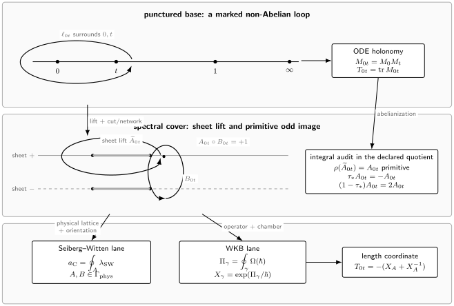
The three cycle carriers in the regular $0t$ frame. The separating loop $\ell_{0t}$ lives on the punctured base and carries the composite matrix $M_0M_t$. A cut or spectral network first produces a literal sheet lift $\widetilde A_{0t}$; a declared filling or quotient and primitive saturation then produce the electric odd class $A_{0t}$ and its conjugate $B_{0t}$. Only after the physical lattice, differential normalization, operator, and analytic chamber are matched may those classes be read as both SW and WKB cycles. Applying $1-\tau_*$ to the already primitive odd class $A_{0t}$ produces $2A_{0t}$.

The weak tube calibrates a primitive odd image

Place the regular singularities at $0,t,1,\infty$, choose the Page 6 base point and counterclockwise generators, and mark the separating loop $\ell_{0t}$ around $0$ and $t$. Its scalar-oper holonomy is

$$M_{0t}=M_0M_t.$$

Now choose a weak-coupling spectral-network chart in which the tube has a closed oriented sheet lift $\widetilde A_{0t}$. Let $\rho$ denote the declared filling or peripheral quotient followed by the physical lattice identification, and define

$$A_{0t} := \rho(\widetilde A_{0t}).$$

Require $A_{0t}$ to be primitive, and choose $B_{0t}$ so that

$$A_{0t}\circ B_{0t}=+1.$$

In the rank-one compact or physical odd sector, the deck involution then acts by

$$\tau_*A_{0t}=-A_{0t}.$$

This equality is not a statement about the two literal embedded sheet lifts in full punctured homology. There, $\widetilde A_{0t}+\tau_*\widetilde A_{0t}$ can be a nonzero invariant peripheral class. The physical lattice passport must say exactly which filling, quotient, and primitive saturation produce $A_{0t}$.

Once $A_{0t}$ is already a primitive odd class, a common normalization trap becomes visible:

$$(1-\tau_*)A_{0t} = 2A_{0t}.$$

Thus the visibly anti-invariant representative obtained by applying $1-\tau_*$ is not primitive here. This is different from an open branch arc $\beta$: the closed chain $\beta-\tau_*\beta$ can itself be primitive, and its period is twice the one-way action. The two factors of two have different origins.

A-period normalization reproduces the composite trace

Use the Page 10 WKB form and normalized period

$$\Omega(\hbar) = P_{\mathrm{ev}}\,\dd z, \qquad \Pi_A := \oint_{A_{0t}}\Omega(\hbar), \qquad a_A^{\mathrm{WKB}} := \frac{\Pi_A}{2\pi\ii}.$$

After the operator, mass, polarization, physical lattice, and scheme passports have been matched, the conditional period dictionary is

$$a_{\mathrm C} \mathrel{\widehat=} a_A^{\mathrm{WKB}}.$$

Page 6 fixed

$$\theta_{0t} = \frac{2a_{\mathrm C}}{\hbar}, \qquad \operatorname{tr}M_{0t} = -2\cos(\pi\theta_{0t})$$

in the natural scalar half-density lift. Substitution gives the normalization audit

$$\begin{aligned} \pi\theta_{0t} &\mathrel{\widehat=} \frac{\Pi_A}{\ii\hbar}, \\ \operatorname{tr}M_{0t} &\mathrel{\widehat=} -2\cos\!\left(\frac{\Pi_A}{\ii\hbar}\right) \\ &= -2\cosh\!\left(\frac{\Pi_A}{\hbar}\right). \end{aligned}$$

The first trace formula is exact for the marked oper and chosen lift. Its final WKB form is a formal identity when $\Pi_A$ is formal. It becomes an analytic statement only when the corresponding exact Abelian coordinate is identified with a specified directional or lateral Borel sum in the same spectral-network chamber.

Equivalently, if

$$X_A := \exp\!\left(\frac{\Pi_A}{\hbar}\right),$$

then the calibrated eigenvalue pair is

$$\operatorname{spec}(M_{0t}) \mathrel{\widehat=} \left\{ -X_A, -X_A^{-1} \right\}.$$

The central minus sign is the scalar half-density contribution; it is not contained in the branch-difference period.

If instead

$$\delta_A := A_{0t}-\tau_*A_{0t} = 2A_{0t},$$

then $\Pi_{\delta_A}=2\Pi_A$ and the same formula reads

$$\operatorname{tr}M_{0t} \mathrel{\widehat=} -2\cosh\!\left( \frac{\Pi_{\delta_A}}{2\hbar} \right).$$

Writing $\Pi_{\delta_A}/\hbar$ would double the monodromy exponent. This one-line test detects whether a source uses a primitive Prym lattice, the image of $1-\tau_*$, or an open one-way action.

The sewing cylinder derives the central sign

At the nodal cusp the internal cylinder reduces to

$$\psi'' + \frac{1-\theta_{0t}^2}{4z^2}\psi = 0, \qquad a_{\mathrm C} = \frac{\hbar\theta_{0t}}2.$$

A basis and its scaled Riccati forms are

$$\begin{aligned} \psi_\pm &= z^{1/2\pm a_{\mathrm C}/\hbar}, \\ \hbar\,\dd\log\psi_\pm &= \left( \frac\hbar2\pm a_{\mathrm C} \right) \frac{\dd z}{z}. \end{aligned}$$

The branch difference is $\Omega=a_{\mathrm C}\,\dd z/z$, so a positive primitive turn gives $\Pi_A=2\pi\ii a_{\mathrm C}$. The mean amplitude term $\hbar\,\dd z/(2z)$ supplies

$$\begin{aligned} \mu_\pm &= \exp\!\left[ 2\pi\ii \left( \frac12\pm\frac{a_{\mathrm C}}\hbar \right) \right] \\ &= -\exp\!\left( \pm\frac{\Pi_A}{\hbar} \right). \end{aligned}$$

This elementary limit derives both the factor $2\pi\ii$ and the central sign.

For the rational Page 6 audit,

$$\hbar=\frac52, \qquad a_{\mathrm C}=\frac34, \qquad \theta_{0t}=\frac35.$$

Hence

$$\Pi_A=\frac{3\pi\ii}{2}, \qquad -2\cosh\!\left(\frac{\Pi_A}{\hbar}\right) = \frac{\sqrt5-1}{2},$$

which is precisely its composite trace. Using the doubled cycle with denominator $\hbar$ would instead give $(1+\sqrt5)/2$ and expose the normalization error.

Four regular punctures give a genus-one audit

For the classical puncture set $X_0$ of a generic regular quadratic differential on the four-punctured sphere, the four double poles force four simple zeros. The normalized double cover branches at those zeros, so Riemann–Hurwitz gives

$$2g(\widehat\Sigma)-2 = 2(-2)+4 = 0, \qquad g(\widehat\Sigma)=1.$$

Each double pole has two unramified preimages. Removing all eight gives

$$\operatorname{rank} H_1(X_0,\mathbb Z) = 2+8-1 = 9.$$

In the generic odd sector, two compact handle directions form the gauge pair $(A,B)$ and four independent odd puncture-loop directions carry flavor residues. Thus its rank is six: a rank-two symplectic gauge sector plus a rank-four flavor radical. The remaining three puncture combinations are invariant. Equivalently,

$$\Gamma_0^- \simeq \mathbb Z_{\mathrm{compact}}^2 \oplus \mathbb Z_{\mathrm{flavor}}^4.$$

On the compact summand, $1-\tau_*$ has image $2\mathbb Z^2$, of index four. The puncture summand has a second saturation effect. If $e_i$ and $f_i$ are the loops over the $i$th pole, then

$$\sum_{i=1}^4(e_i+f_i)=0.$$

Every difference $e_i-f_i$ lies in the image of $1-\tau_*$, but the odd class

$$v:=\sum_{i=1}^4e_i$$

satisfies

$$2v = \sum_{i=1}^4(e_i-f_i).$$

Thus the four differences span an index-two sublattice of the saturated odd puncture lattice. Altogether,

$$\left[ \Gamma_0^-: (1-\tau_*)H_1(X_0,\mathbb Z) \right] = 8.$$

At WKB order $N\geq1$, the standard puncture set also removes the four ramification points because higher WKB coefficients have poles there. Then there are twelve punctures and $\operatorname{rank}H_1(X_N,\mathbb Z)=13$. Those four new peripheral loops are fixed by $\tau_*$, so the odd rank remains six while the invariant rank becomes seven. The new invariant puncture relation removes the parity class $v$ from the odd kernel. In fact the deck action on $X_N$ is now free and

$$\ker(1+\tau_*) = \operatorname{im}(1-\tau_*) \subset H_1(X_N,\mathbb Z).$$

Thus the full punctured WKB lattice has image index one. If the ramification punctures are filled again before projecting to a compact odd target, the compact factor-of-four saturation reappears. The puncture convention is therefore part of any quoted index.

These rank matches are structural, but they still do not prove that the physical charge lattice is the entire odd lattice; global form can change it by finite index or a quotient.

The plumbing limit $t\to0$ is also not a Coulomb discriminant. The base tube can become long while locally

$$\Omega_0 \simeq a_{\mathrm C}\frac{\dd w}{w},$$

so its normalized electric period remains finite; the dual period develops the weak-coupling logarithm. A pinched ultraviolet sewing tube does not by itself imply that a BPS charge becomes massless.

The reverse trace map needs five passports

Before inverting even a nonresonant trace, restore five kinds of data.

Passport	What must be supplied	Failure without it
Projection	Branched cover, punctures, ramification, and an embedded representative	An abstract odd class does not determine a base loop
Cut or network	Sheet choice, detours, gluing, $\mathcal W$-framing, and the twisting or ramification-holonomy convention	Abelian holonomies do not reconstruct non-Abelian holonomy
Integral lattice	$\ker(1+\tau_*)$ versus $\operatorname{im}(1-\tau_*)$, primitive saturation, physical sublattice, and flavor quotient	Charge units and factors of two remain undetermined
Orientation and marking	Base stem and word order, sheet or eigenline, cycle orientation, and $A\circ B$ sign	Signs, inverse eigenvalues, and electric–magnetic labels remain ambiguous
Analytic chamber	Borel ray, lateral side, Stokes graph, logarithm sheet, and continuation path	A formal Voros symbol does not select an analytic coordinate

Let $T_{0t}=\operatorname{tr}M_{0t}$. Away from $T_{0t}=\pm2$, define an Abelian length coordinate $X_A$ by

$$T_{0t} = -\left(X_A+X_A^{-1}\right).$$

The quadratic equation gives reciprocal roots. Recovering an additive period then requires

$$X_A = \exp\!\left(\frac{\Pi_A}{\hbar}\right), \qquad \frac{\Pi_A}{\hbar} = \pm\operatorname{arcosh}\!\left(-\frac{T_{0t}}2\right) +2\pi\ii k,$$

with $k\in\mathbb Z$. The signs exchange the two eigenlines or reverse $A$; the integer changes the logarithm sheet. A determinant-one lift of the projective monodromy fixes the remaining central sign. Finally, one must know whether the recovered class is primitive in $\Gamma_{\mathrm{phys}}$.

At $T_{0t}=\pm2$, the roots coincide. The trace cannot distinguish $I$ from a nontrivial unipotent block when $T_{0t}=2$, or $-I$ from a negative-unipotent block when $T_{0t}=-2$, and $\operatorname{arcosh}$ is ramified. The correct inverse datum is the full conjugacy class together with a limiting eigenline or Jordan flag—not a chosen square root of the trace discriminant.

The conjugate twist belongs to the B-lane

The marked four-puncture character variety has two local dimensions after the four local conjugacy classes are fixed. The classical-block generating-function page and Page 6 used the length coordinate $\theta_{0t}$ and a conjugate twist $\mu_{0t}$, normalized by

$$\dd W = c_t^{\mathrm{op}}\,\dd t + \mu_{0t}\,\dd\theta_{0t}.$$

The A-period fixes the length lane. The B-period can represent the twist lane only after a full generating function has been chosen. To see the factor in the book’s convention, suppose that the normalized oper generator and the local gauge NS generator obey

$$W(\theta_{0t},t) \mathrel{\widehat=} \frac{1}{\hbar} \widetilde{\mathcal W}_{\mathrm{NS}}(a_{\mathrm C},t), \qquad \theta_{0t} = \frac{2a_{\mathrm C}}{\hbar}.$$

Then

$$\mu_{0t} \mathrel{\widehat=} \frac12 \frac{\partial \widetilde{\mathcal W}_{\mathrm{NS}}} {\partial a_{\mathrm C}}.$$

If the same normalization also satisfies the Page 10 quantum special-geometry relation

$$a_D^{\mathrm{WKB}} \mathrel{\widehat=} -\frac{\hbar}{2\pi\ii} \frac{\partial \widetilde{\mathcal W}_{\mathrm{NS}}} {\partial a_{\mathrm C}}, \qquad \Pi_B=2\pi\ii a_D^{\mathrm{WKB}},$$

then the house conversion is

$$\mu_{0t} \mathrel{\widehat=} -\frac{\Pi_B}{2\hbar}.$$

This is a derived conditional formula, not a universal definition of a Fenchel–Nielsen twist. Adding a $t$-independent term $W_0(\theta_{0t})$ leaves $c_t^{\mathrm{op}}$ unchanged but sends

$$\mu_{0t} \longmapsto \mu_{0t}+W_0'(\theta_{0t}).$$

On the gauge side the same freedom is a perturbative, boundary, or scheme term that shifts the dual derivative. An accessory match thus does not calibrate the B-lane.

Under the same hypotheses, the multiplicative B-coordinate is

$$X_B := \exp\!\left(\frac{\Pi_B}{\hbar}\right) \mathrel{\widehat=} \exp\!\left( -\frac{\partial \widetilde{\mathcal W}_{\mathrm{NS}}} {\partial a_{\mathrm C}} \right).$$

It is generally not the trace of a second simple base loop. The other pair traces on the four-puncture character variety are rational or Laurent expressions in $X_A$, $X_B$, and the four local monodromy eigenvalues.

Reversible dictionary: carriers and lifts

The following tables make “corresponds to” operational. A reverse arrow means that the listed restoration data are part of the input; it never means that a printed number determines an embedded cycle by itself.

Map	Forward direction	Reverse direction	Convention and excluded cases	Primary source
Based loop $\leftrightarrow$ ODE holonomy	Continue a normalized fundamental matrix along $\ell$ to obtain $M_\ell$	Recover the representation from a marked generating set satisfying the puncture product relation and prescribed local conjugacy classes, modulo simultaneous conjugation	Fix $z_*$, loop order, orientation, and an $SL(2)$ lift; a single trace is insufficient, especially at trace $\pm2$	Nekrasov–Rosly–Shatashvili, §§2–3
Base local system $\leftrightarrow$ Abelian cover data	Abelianize on the open locus of $\mathcal W$-framed connections, including every detour across network walls	Apply the local non-Abelianization map with the same network and gluing rules	Requires a nondegenerate network, fixed puncture holonomies, flags, cover, and twisting; it is not a global bijection	Gaiotto–Moore–Neitzke, §§9–10; Hollands–Neitzke, §2.4
Marked tube $\leftrightarrow$ primitive odd image	Lift $\ell_{0t}$ to $\widetilde A_{0t}$, then apply the declared filling or quotient and primitive saturation to obtain $A_{0t}$	Restore the physical embedding, a literal sheet lift, sheet, cuts, tube marking, and detours	The sheet lift must close; $(1-\tau_*)A=2A$ only when $A$ is already primitive and odd	Hollands–Kidwai, §2.1 and §§5–7
Cover homology $\leftrightarrow$ physical SW charge	Select the integral electromagnetic or Prym lattice and its flavor radical inside the cover topology	Restore the embedding or quotient, polarization, and charge normalization from the physical theory	Work off the discriminant; not every class in $H_1$ is physical or primitive	Seiberg–Witten, §6; Gaiotto–Moore–Neitzke, §3.1.4
SW class $\leftrightarrow$ WKB class	Match the principal-symbol cover, oriented integral frame, and leading one-form	Restore the operator ordering, half-form, puncture set, and regularization	Equality of classical curves alone is insufficient; turning-point collisions and higher-order WKB poles require limiting data	Hollands–Kidwai, §2.1 and §11; Hollands–Neitzke, §§2–3

The second table concerns coordinates carried by those objects.

Map	Forward direction	Reverse direction	Convention and excluded cases	Primary source
Composite matrix $\leftrightarrow$ trace	$M_{0t}\mapsto T_{0t}=\operatorname{tr}M_{0t}$	Recover a generic conjugacy class after choosing the semisimple or Jordan type; an actual based matrix and full representation require framing and the other generators	At $T_{0t}=\pm2$, trace does not determine semisimple versus unipotent monodromy	Litvinov–Lukyanov–Nekrasov–Zamolodchikov, §2
Trace $\leftrightarrow$ exponent	$\theta_{0t}\mapsto-2\cos(\pi\theta_{0t})$	Choose $\theta_{0t}$ modulo $\theta\mapsto\pm\theta+2k$ and restore the scalar lift	The inverse is ramified when the trace is $\pm2$; logarithmic or Jordan information must be added	Jeong–Nekrasov, §5.2.1 and §6.1
Exponent $\leftrightarrow$ Coulomb coordinate	$a_{\mathrm C}\mapsto\theta_{0t}=2a_{\mathrm C}/\hbar$	$a_{\mathrm C}=\hbar\theta_{0t}/2$ after the Omega plane and Weyl representative are fixed	Exclude $\hbar=0$ as an inverse formula; at $a_{\mathrm C}=0$ the Weyl quotient is ramified	Alday–Gaiotto–Tachikawa, §3; Jeong–Nekrasov, §6.1
Coulomb coordinate $\leftrightarrow$ A-period	$a_{\mathrm C}\mathrel{\widehat=}\Pi_A/(2\pi\ii)$	Select the primitive $A$, quantum mirror-map branch, curve differential, and Gauss–Manin path	Conditional WKB–NS map; fails as a coordinate where $\partial_u\Pi_A=0$; at a discriminant the homology frame needs limiting transport data	Hollands–Kidwai, §2.1 and §11.3
Twist $\leftrightarrow$ B-period	$\mu_{0t}\mathrel{\widehat=}-\Pi_B/(2\hbar)$ in the house normalization	Restore $W_0$, the $A\circ B=+1$ polarization, perturbative scheme, and logarithm branch	Not defined by accessory data alone; avoid singular Darboux charts and resonant length coordinates	Nekrasov–Rosly–Shatashvili, §§3–4; Jeong–Nekrasov, §6.1; Hollands–Kidwai, §§11.2–11.3
Additive WKB period $\leftrightarrow$ Voros symbol	$\Pi_\gamma\mapsto\mathcal V_\gamma=\exp(\Pi_\gamma/\hbar)$	Choose a logarithm sheet and add $2\pi\ii\hbar k$	Formal exponentiation is always algebraic; analytic inversion additionally needs a Borel direction and lateral side	Iwaki–Nakanishi, §§2–3

The hats in the period rows carry real content. They abbreviate the operator, differential, lattice, scheme, mirror-map, and analytic gates listed explicitly on the Chapter 10 period page. They do not mean “equal up to an unimportant convention.”

Five transformations must remain separate

The word “monodromy” is overloaded independently of “cycle,” and a graph-basis mutation is often folded into the same formula despite being a separate relabeling.

Operation	What is moved	What changes	What stays fixed
ODE monodromy	The probe coordinate around a based loop in $C^\circ$	The solution frame through $M_\ell$	Operator parameters
Mapping-class or S-duality action	Puncture marking and sewing chart	Pants channel, trace coordinates, gauge frame, and flavor basis	The global theory after transport
Gauss–Manin monodromy	A modulus around a discriminant in $\mathcal B^\circ$	The integral SW/WKB cycle frame and its period vector	The geometrically transported charge section
Exact-WKB Stokes automorphism	The Borel direction across a singular ray	Lateral Voros coordinates	The exact ODE local system
Stokes-graph basis mutation	The preferred network-adapted basis	The coordinate chart and labels	The fixed lattice after a separate transport identification

In particular, the Picard–Lefschetz matrix acting on $(A,B)$ is not the solution matrix $M_0M_t$. A fixed-lattice Stokes jump is also not the same operation as relabeling the graph basis, even when both appear in one cluster-mutation formula.

Frame changes act on the whole passport

A cycle basis is a local frame of an integral local system, not a set of permanent names. Three superficially similar changes occur in the three languages.

Change	ODE or character-variety effect	SW effect	WKB effect
Reverse both cycles	Exchange the chosen eigenvalue representative while preserving the composite trace	$(A,B)\mapsto(-A,-B)$ and $(a,a_D)\mapsto(-a,-a_D)$	$(\Pi_A,\Pi_B)\mapsto(-\Pi_A,-\Pi_B)$; Voros symbols invert
Dehn twist about $A$	Shift the twist coordinate while keeping the length coordinate fixed	$B\mapsto B+kA$, so $a_D\mapsto a_D+ka$	$\Pi_B\mapsto\Pi_B+k\Pi_A$ in the transported chamber
Change pants decomposition	Replace the chosen composite loop and length–twist chart	Change electric–magnetic duality frame	Replace the preferred WKB basis, generally after continuation
Cross a finite Stokes wall	Keep the non-Abelian local system fixed	Keep the transported physical charge lattice, although BPS coordinates may jump	Mutate the spectral coordinates by the Stokes or cluster automorphism
Circle a discriminant component	Analytically continue the character data	Apply integral Gauss–Manin or electromagnetic monodromy	Transport cycles and resummed coordinates along the same path

For example, the rank-one Dehn twist

$$\begin{pmatrix} A'\\ B' \end{pmatrix} = \begin{pmatrix} 1&0\\ k&1 \end{pmatrix} \begin{pmatrix} A\\ B \end{pmatrix}$$

preserves $A\circ B=+1$ and yields

$$\Pi_A'=\Pi_A, \qquad \Pi_B'=\Pi_B+k\Pi_A.$$

Under the conditional house conversion, the twist changes by

$$\mu_{0t}' = \mu_{0t} - \frac{k\Pi_A}{2\hbar}.$$

This is not a contradiction with the invariant composite trace: the length coordinate has not changed. It is the expected canonical ambiguity in the conjugate coordinate.

At a Stokes wall, the Voros-symbol transformation is nonlinear after exponentiation. For a saddle class $\gamma_0$, a typical lateral jump has the schematic form

$$\mathcal V_\gamma^+ = \mathcal V_\gamma^- \left( 1+\mathcal V_{\gamma_0}^- \right)^{\langle\gamma_0,\gamma\rangle},$$

with the sign and exponent convention fixed by the exact-WKB setup. One must transform every spectral coordinate used to reconstruct $M_\ell$. Comparing $\mathcal V_A$ on one side of the wall with $\mathcal V_B$ on the other while leaving the reconstruction formula unchanged mixes charts.

Absolute cycles and relative paths answer different questions

Closed electromagnetic charges and WKB periods do not exhaust the connection problem. A normalized connection coefficient often uses an open path

$$\beta \in H_1(X_N,E;\mathbb Z),$$

whose endpoint set $E$ contains turning points, puncture lifts, or chosen normalization points. Its regularized integral depends on endpoint conventions that no closed charge records.

The distinctions are:

Object	Boundary	Typical use	Extra data
Absolute cover cycle $\gamma$	$\partial\gamma=0$	SW central charge, closed WKB period, Voros multiplier	Primitive lattice, orientation, puncture set
Relative WKB path $\beta$	$\partial\beta\in E$	Tunneling action or connection coefficient	Endpoint local coordinate, subtraction, normalization
Small puncture loop $\ell_p$	Closed after removing $p$	Mass or residue period	Positive orientation and residue convention
Based loop on $C^\circ$	Begins and ends at $z_*$	Non-Abelian analytic continuation	Base point, ordered word, fundamental matrix

If $\beta$ joins two branch points, the anti-invariant closure

$$\delta_\beta = \beta-\tau_*\beta$$

may be a primitive absolute cycle. Because $\Omega$ is anti-invariant,

$$\oint_{\delta_\beta}\Omega = 2\int_\beta\Omega.$$

This legitimate factor of two must not be confused with applying $1-\tau_*$ to an already closed primitive cycle. Page 8’s normalization-complete connection example will use relative paths and endpoint bases explicitly.

Where the generic dictionary stops

The map is local on the complement of several exceptional divisors and walls.

Locus	What ceases to be generic	Required replacement
Local exponent difference in $\mathbb Z$	Frobenius eigenbasis can become logarithmic	Resonant basis, limiting connection matrix, and Jordan data
Composite trace $T_{0t}=\pm2$	Length coordinate and trace inverse ramify	Full conjugacy class plus limiting eigenline or Jordan flag
SW discriminant	A charge cycle vanishes geometrically and the fixed homology frame degenerates	Picard–Lefschetz/Gauss–Manin limiting data and, when needed, another local frame
Turning-point collision	The WKB cover or simple-turning-point graph degenerates	Uniform local model and a recomputed puncture/relative-homology problem
Critical spectral network	Abelianization chart reaches a wall	Lateral chart, mutation, or limiting network with detours retained
Borel singular direction	One formal Voros symbol has two lateral sums	Specify $\mathcal S_{\vartheta+}$ or $\mathcal S_{\vartheta-}$ and apply the Stokes automorphism
Nonprimitive or quotient charge	Cover period has the wrong integral normalization	State the physical sublattice or quotient and recalibrate the factor
$\partial_u\Pi_A=0$	The A-period is not a local coordinate	Change special coordinate or use a ramified mirror map

Resonance is not one condition shared by all rows. A local Frobenius resonance concerns an external exponent; trace resonance concerns the composite length; a discriminant concerns the spectral curve; and a Stokes wall concerns an analytic summation chart. Their remedies should not be interchanged.

A cycle passport that can be rerun backward

Before translating a connection problem, record the following data in one place.

1. Base carrier: $C^\circ$, its punctures, $z_*$, oriented loop generators, and the marked composite word.
2. Monodromy lift: projective versus $SL(2)$ normalization, fundamental-matrix normalization, eigenvalue logarithms, and Jordan data at resonance.
3. Spectral cover: the normalized equation for $\widehat\Sigma$, projection $\pi$, deck involution $\tau$, and branch cuts.
4. Abelianization chart: WKB phase or spectral network, detour rules, $\mathcal W$-framing, twisting or ramification holonomy, and its nondegeneracy chamber.
5. Integral lattice: primitive cover classes, the physical charge sublattice or quotient, flavor radical, and the distinction between $A$ and $(1-\tau_*)A$.
6. Polarization: orientations and intersections, especially $A\circ B=+1$, plus the Gauss–Manin continuation path.
7. Forms and factors: $\lambda_{\mathrm{SW}}$, $\Omega(\hbar)$, the $2\pi\ii$ normalization, half-form convention, and residue or endpoint regularization.
8. Gauge and CFT data: Omega plane, Weyl representative, internal momentum lift, full generating-function normalization, and perturbative or boundary scheme.
9. Analytic realization: formal versus Borel-resummed quantities, Borel ray, lateral side, Stokes chamber, and logarithm sheet.
10. Failure audit: local and composite resonances, discriminant components, turning-point collisions, and mirror-map critical points excluded from the claimed domain.

With this passport, the forward route

$$\ell_{0t} \longrightarrow M_{0t} \longrightarrow \theta_{0t} \longrightarrow a_{\mathrm C} \mathrel{\widehat=} \frac{\Pi_A}{2\pi\ii}$$

and its reverse are statements with checkable inputs. Without it, the same chain is only mnemonic notation.

Common pitfalls

Drawing the base loop on the SW curve. The monodromy loop lives on $C^\circ$; the charge lives on $\widehat\Sigma$. Draw the projection map and specify the sheet lift or abelianization network between them.

Antisymmetrizing twice. A primitive closed class with $\tau_*A=-A$ is already anti-invariant. Applying $1-\tau_*$ produces $2A$ and doubles every period unless the denominator is corrected.

Calling a trace a period. A trace is invariant under eigenvalue inversion and periodic shifts of its logarithm. Recovering a period requires a determinant-one lift, eigenvalue branch, primitive cycle, and logarithm sheet.

Using accessory agreement to fix the B-period. A $t$-independent term in the generating function leaves the accessory unchanged and shifts the conjugate twist. The perturbative and boundary normalization must be audited separately.

Holding cycle labels fixed across a wall. A Stokes graph or duality frame change transforms the coordinates and their reconstruction formula together. “A-cycle” on two sides of a wall need not denote the same transported class.

Using a relative action as a closed charge. An open path carries endpoint subtractions and basis normalizations. Close it explicitly and track the factor of two before comparing it with an SW period.

Exercises

1. Identify the carrier

Classify each object as a base loop, an absolute cover cycle, a relative cover path, or a number carried by one of them: $\ell_{0t}$, $M_0M_t$, $A_{0t}$, $\Pi_A$, $\beta$, and $\mathcal V_A$.

Solution

$\ell_{0t}$ is a based loop on $C^\circ$, and $M_0M_t$ is its non-Abelian holonomy matrix. $A_{0t}$ is an absolute cover cycle and $\Pi_A$ its additive period. $\beta$ denotes a relative cover path. $\mathcal V_A$ is the exponentiated period carried by $A_{0t}$; it is not itself a cycle.

2. Audit a closed lift

Suppose $A$ is primitive and $\tau_*A=-A$. Express $\Pi_{A-\tau_*A}$ in terms of $\Pi_A$ and write the correct trace formula using the antisymmetrized class.

Solution

In homology,

$$A-\tau_*A=2A, \qquad \Pi_{A-\tau_*A}=2\Pi_A.$$

Therefore

$$\operatorname{tr}M_{0t} \mathrel{\widehat=} -2\cosh\!\left( \frac{\Pi_{A-\tau_*A}}{2\hbar} \right).$$

3. Derive the A-period trace

Starting from $a_{\mathrm C}=\Pi_A/(2\pi\ii)$, $\theta_{0t}=2a_{\mathrm C}/\hbar$, and $\operatorname{tr}M_{0t}=-2\cos(\pi\theta_{0t})$, derive the hyperbolic-cosine formula.

Solution

The first two relations give

$$\pi\theta_{0t} = \frac{\Pi_A}{\ii\hbar}.$$

Since $\cos(x/\ii)=\cosh x$,

$$\operatorname{tr}M_{0t} = -2\cosh\!\left(\frac{\Pi_A}{\hbar}\right).$$

The equality is formal or analytic according to the status of the WKB–SW period identification.

4. Invert a nonresonant trace

Let $T_{0t}=3$. Describe all additive Abelian lengths compatible with $T_{0t}=-(X_A+X_A^{-1})$ and $X_A=\exp(\Pi_A/\hbar)$.

Solution

The two reciprocal roots are

$$X_A = \frac{-3\pm\sqrt5}{2}.$$

For either root and any $k\in\mathbb Z$,

$$\frac{\Pi_A}{\hbar} = \log X_A+2\pi\ii k.$$

Equivalently these are the branches $\pm\operatorname{arcosh}(-3/2)+2\pi\ii k$. An orientation or eigenline choice selects the sign, and a logarithm sheet selects $k$.

5. Transport through a Dehn twist

For $B'=B+2A$, compute $\Pi_B'$ and the corresponding change of $\mu_{0t}$ in the house B-lane normalization.

Solution

Linearity of periods gives

$$\Pi_B'=\Pi_B+2\Pi_A.$$

Using $\mu_{0t}=-\Pi_B/(2\hbar)$,

$$\mu_{0t}' = \mu_{0t}-\frac{\Pi_A}{\hbar}.$$

The A-period and composite trace remain fixed.

6. Detect the invisible B-lane shift

Let $W\mapsto W+g(\theta_{0t})$. Which quantities on this page change?

Solution

Because $g$ is independent of $t$, $c_t^{\mathrm{op}}=\partial_tW$ does not change. The twist does:

$$\mu_{0t} \longmapsto \mu_{0t}+g'(\theta_{0t}).$$

Consequently a B-period identified with the twist must shift in the matched scheme, while the A-period, internal exponent, and composite trace are unchanged.

7. Close a one-way action

Let $\beta$ be an oriented path between two branch points and assume $\delta_\beta=\beta-\tau_*\beta$ is primitive. Show how its closed period compares with the one-way action.

Solution

Anti-invariance gives

$$\int_{\tau_*\beta}\Omega = -\int_\beta\Omega.$$

Hence

$$\oint_{\delta_\beta}\Omega = \int_\beta\Omega - \int_{\tau_*\beta}\Omega = 2\int_\beta\Omega.$$

Here the factor two compares a closed period with an open one-way action; it does not signal that $\delta_\beta$ is nonprimitive.

8. Explain why trace resonance needs more data

Give two nonconjugate determinant-one matrices with trace $2$ and state the missing datum.

Solution

For example,

$$I \qquad\text{and}\qquad \begin{pmatrix} 1&1\\0&1 \end{pmatrix}$$

both have determinant one and trace $2$, but the first is semisimple and the second is a nontrivial unipotent Jordan block. The trace must be supplemented by the conjugacy type and, for a limiting inverse map, an eigenline or Jordan flag.

References

• N. Seiberg and E. Witten, “Electric–Magnetic Duality, Monopole Condensation, and Confinement in N=2 Supersymmetric Yang–Mills Theory”, Nuclear Physics B 426 (1994), 19–52; erratum 430 (1994), 485–486. Section 6 identifies electric and magnetic special coordinates with periods of a distinguished differential and tracks their monodromy.
• D. Gaiotto, “N=2 Dualities”, Journal of High Energy Physics 08 (2012) 034. Sections 2–3 construct the class-$S$ curve, pants-decomposition frames, and the corresponding charge and period geometry.
• N. Nekrasov, A. Rosly, and S. Shatashvili, “Darboux Coordinates, Yang–Yang Functional, and Gauge Theory”, Nuclear Physics B Proceedings Supplements 216 (2011), 69–93. Sections 2–4 define holomorphic length–twist coordinates on character varieties and propose the oper-locus/Yang–Yang generating-function identification, with its normalization dependence visible.
• D. Gaiotto, G. W. Moore, and A. Neitzke, “Wall-Crossing, Hitchin Systems, and the WKB Approximation”, Advances in Mathematics 234 (2013), 239–403. Section 3.1.4 separates the spectral-cover homology from the physical charge subquotient and its flavor radical; Section 7 relates WKB triangulations to charge coordinates and their intersections.
• D. Gaiotto, G. W. Moore, and A. Neitzke, “Spectral Networks”, Annales Henri Poincaré 14 (2013), 1643–1731. Section 9 defines the path lifting and detour rules; Section 10 constructs the local non-Abelianization map and spectral coordinates, without asserting a global inverse equivalence.
• K. Iwaki and T. Nakanishi, “Exact WKB Analysis and Cluster Algebras”, Journal of Physics A 47 (2014) 474009. Sections 2–3 define path and cycle Voros symbols; later sections derive their Stokes-graph mutations and associated automorphisms.
• L. Hollands and O. Kidwai, “Higher Length-Twist Coordinates, Generalized Heun’s Opers, and Twisted Superpotentials”, 2017. Section 2.1 gives the four-puncture spectral curve and periods; Sections 3–4 define Fenchel–Nielsen-type networks and length–twist coordinates; Sections 5–7 realize them by abelianization; and Section 11 compares the NRS and exact-WKB or quantum-period descriptions.
• S. Jeong and N. Nekrasov, “Opers, Surface Defects, and Yang–Yang Functional”, Advances in Theoretical and Mathematical Physics 24 (2020), 1789–1916. Sections 5.2.1 and 6.1, especially equations (5.38), (6.11), and (6.24)–(6.25), give the four-puncture composite length, its conjugate coordinate, and the normalization-complete oper generating function used in the Chapter 11 calibration.
• L. Hollands and A. Neitzke, “Exact WKB and Abelianization for the T₃ Equation”, Communications in Mathematical Physics 380 (2020), 131–186. Sections 2–3 explain exact WKB as abelianization and relate spectral coordinates to quantum-period asymptotics, including the dependence on WKB phase.
• D. G. L. Allegretti, “Voros Symbols as Cluster Coordinates”, Journal of Topology 12 (2019), 1031–1068. Theorems 1.3 and 7.13 identify Borel-summed cycle Voros symbols with Fock–Goncharov coordinates for complete saddle-free signed and marked differentials under the stated half-plane hypotheses; Theorem 7.13 is the proof of the result announced as Theorem 1.3.
• A. Litvinov, S. Lukyanov, N. Nekrasov, and A. Zamolodchikov, “Classical Conformal Blocks and Painlevé VI”, Journal of High Energy Physics 07 (2014) 144. Section 2 gives the four-puncture oper, composite monodromy trace, and classical generating-function framework underlying the length lane.