Analytic Continuation and Monodromy Representations

A local solution germ becomes a global analytic object only after its continuations along all admissible paths are organized. The central object is the monodromy representation, but it is not the whole connection problem: local normalizations, paths between them, Stokes factors at irregular points, and boundary conditions carry information that an ordinary monodromy conjugacy class forgets.

This chapter answers:

Chapter question

How do normalized local or sectorial solutions assemble into a global analytic object, and which part of that object is selected by a boundary, scattering, resonance, or spectral problem?

The prerequisites are the local-system toolkit, the book’s right-action conventions, and the Chapter 1 case files. This page starts with ordinary analytic continuation. The rest of the chapter adds irregular, connection, moduli, and operator-theoretic data without changing the conventions fixed here.

From germs to the universal cover

Let $\Sigma$ be a connected Riemann surface, let

$$D=\{a_1,\ldots,a_m\}, \qquad X=\Sigma\setminus D,$$

and let $(E,\nabla)$ be a rank-$n$ holomorphic flat bundle on $X$. In a local coordinate and bundle trivialization, write $\nabla=\dd-\Omega$ with

$$\dd Y=\Omega Y, \qquad \Omega=A(z)\,\dd z.$$

Choose a base point $z_*\in X$, a frame of $E_{z_*}$, and the normalized fundamental matrix $\Phi(z_*)=I$. Analytic continuation through local trivializations makes $\Phi$ single-valued on the universal cover $\widetilde X$, while a deck transformation associated with a based loop $\gamma$ produces another fundamental matrix $\Phi^\gamma$.

Both matrices solve the same system. Therefore

$$\begin{aligned} \frac{\dd}{\dd z} \left( \Phi^{-1}\Phi^\gamma \right) &= -\Phi^{-1}A\Phi\, \Phi^{-1}\Phi^\gamma +\Phi^{-1}A\Phi^\gamma\\ &=0. \end{aligned}$$

Their ratio is constant:

$$\Phi^\gamma=\Phi M_\gamma, \qquad M_\gamma\in GL(n,\mathbb C).$$

The matrix is not attached to the geometric circle alone. It depends on its based homotopy class and on the ordered frame $\Phi(z_*)$.

Path order fixes matrix order

The book uses the composition in which $\gamma_1\gamma_2$ traverses $\gamma_2$ first and then $\gamma_1$. Successive continuation gives

$$\Phi^{\gamma_1\gamma_2} = \left( \Phi^{\gamma_2} \right)^{\gamma_1} = \Phi M_{\gamma_1}M_{\gamma_2},$$

so

$$\rho_\Phi: \pi_1(X,z_*)\longrightarrow GL(n,\mathbb C), \qquad \rho_\Phi(\gamma)=M_\gamma$$

is a representation with

$$M_{\gamma_1\gamma_2} = M_{\gamma_1}M_{\gamma_2}.$$

In a trivialization along a parametrized loop, the same matrix is

$$M_\gamma = \mathcal P \exp\left[ \int_0^1 A(\gamma(t))\gamma'(t)\,\dd t \right],$$

where path ordering places later times on the left. The symbol $\mathcal P$ cannot be dropped when coefficient matrices at different points fail to commute.

This convention is easy to audit: the matrix written farther left belongs to the path traversed later. Sources using “first $\gamma_1$, then $\gamma_2$” reverse the path product before their formulas can be compared with ours.

The monodromy group is only the image $\rho_\Phi(\pi_1(X,z_*))$. It forgets which based loop maps to which matrix, whereas the monodromy representation retains that marking.

On the punctured sphere, choose a distinguished system of positively oriented based loops and label it so that

$$\gamma_1\gamma_2\cdots\gamma_m=1.$$

Then

$$M_1M_2\cdots M_m=I.$$

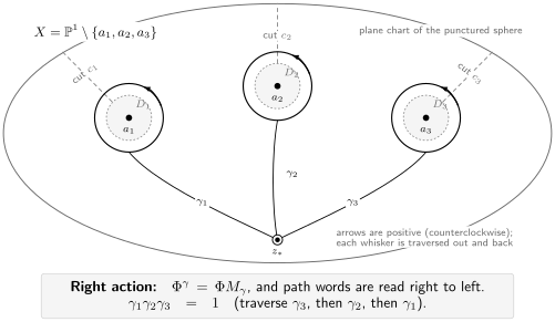
A distinguished system of based positive loops. With the book’s path composition, $\gamma_1\gamma_2\gamma_3=1$ is traversed from right to left, and the right-acting matrices obey $M_1M_2M_3=I$.

The relation belongs to the chosen generators. Moving the base point, changing the tails of the loops, or braiding punctures changes the displayed tuple even when the underlying local system is unchanged.

Frames, gauges, and conjugacy

Three transformations that look similar in a formula act differently on monodromy.

Changing the solution frame

Replace the normalized frame by

$$\widetilde\Phi=\Phi H, \qquad H\in GL(n,\mathbb C).$$

Then

$$\widetilde\Phi^\gamma = \widetilde\Phi \left( H^{-1}M_\gamma H \right),$$

and hence

$$\widetilde M_\gamma = H^{-1}M_\gamma H.$$

Without a preferred frame, the invariant object is therefore the simultaneous conjugacy class of the representation. Individual entries become meaningful only after a normalization has been fixed.

Applying a single-valued gauge

For a single-valued invertible left gauge $G(z)$, set

$$\widetilde\Phi(z)=G(z)\Phi(z).$$

If the same solution frame is retained, then

$$\widetilde\Phi^\gamma = G\Phi^\gamma = \widetilde\Phi M_\gamma.$$

The numerical right monodromy matrices do not change. By contrast, a multivalued scalar gauge with

$$g^\gamma=\chi(\gamma)g$$

twists the representation:

$$\widetilde M_\gamma = \chi(\gamma)M_\gamma.$$

This is why removing the first derivative locally can preserve projective monodromy while changing a chosen $GL(2)$ lift.

Transporting a local frame

Suppose a local normalized frame $\Phi_i$ and the continued base frame $\Phi_*$ meet on a common branch, with

$$\Phi_i=\Phi_*C_{*i}.$$

If the positive local loop has matrix $D_i$ in $\Phi_i$, its based monodromy in the $\Phi_*$ frame is

$$M_i^{(*)} = C_{*i}D_iC_{*i}^{-1}.$$

The connection matrix is therefore not auxiliary decoration: it embeds local monodromy into the common global frame. Its path, direction, bases, and branches must be recorded next to it.

Abel’s determinant audit

For the scalar equation

$$y''+p(z)y'+q(z)y=0,$$

use the companion fundamental matrix

$$\Phi = \begin{pmatrix} y_1&y_2\\ y_1'&y_2' \end{pmatrix}.$$

Its determinant is the book’s Wronskian:

$$\det\Phi=\Wr[y_1,y_2].$$

Abel’s identity gives

$$\Wr'=-p\,\Wr.$$

After continuation around $\gamma$,

$$\frac{\Wr^\gamma}{\Wr} = \det M_\gamma,$$

while integration of Abel’s equation gives the exact audit

$$\det M_\gamma = \exp\left( -\oint_\gamma p(z)\,\dd z \right).$$

For a positive loop around a single meromorphic point $a_i$,

$$\det M_i = \exp\left[ -2\pi\ii\operatorname{Res}_{a_i}p \right].$$

At a regular singularity the indicial roots obey

$$\rho_++\rho_- = 1-\operatorname{Res}_{a_i}p.$$

Thus the determinant computed from the Frobenius eigenvalues is

$$\ee^{2\pi\ii(\rho_++\rho_-)} = \ee^{-2\pi\ii\operatorname{Res}_{a_i}p},$$

in agreement with Abel’s identity. This check detects a reversed loop, a missing scalar gauge factor, or an inconsistent lift before a full matrix calculation is attempted.

A logarithm remembers more than eigenvalues

Consider

$$y''+\frac1z y'=0$$

on the principal branch near the positive real axis. An ordered fundamental matrix is

$$\Phi(z) = \begin{pmatrix} 1&\operatorname{Log}z\\ 0&z^{-1} \end{pmatrix}.$$

A positive loop sends

$$\operatorname{Log}z \longmapsto \operatorname{Log}z+2\pi\ii,$$

so

$$M_0 = \begin{pmatrix} 1&2\pi\ii\\ 0&1 \end{pmatrix}.$$

Both eigenvalues equal $1$, but the monodromy is not the identity and is not semisimple. The eigenvalues remember the exponents only modulo integers; the Jordan part records the logarithmic obstruction.

The determinant audit also works:

$$\operatorname{Res}_0p=1, \qquad \det M_0=\ee^{-2\pi\ii}=1.$$

It confirms the determinant, but it cannot distinguish this unipotent matrix from $I$. Trace and determinant are not a complete substitute for the full matrix at reducible or resonant points.

This example also shows why one must not write $M_\gamma=\exp\oint_\gamma A\,\dd z$. Its companion matrix is

$$A(z) = \begin{pmatrix} 0&1\\ 0&-z^{-1} \end{pmatrix}.$$

The exponential of its ordinary contour integral is $I$, while the path-ordered exponential is the nontrivial unipotent matrix above.

Projective monodromy

For two scalar solutions write $w=y_1/y_2$. If

$$M_\gamma = \begin{pmatrix} a&b\\ c&d \end{pmatrix},$$

then the right-action convention gives

$$w^\gamma = \frac{aw+c}{bw+d}.$$

Only the class of $M_\gamma$ in $PGL(2,\mathbb C)$ acts on $w$. This is the projective monodromy naturally associated with the oper ratio. It is a right action on the row projective coordinate $w=y_1/y_2$; sources using column coordinates display the transposed Möbius coefficients.

Trivial monodromy need not mean an ordinary point

The equation

$$y''-\frac2z y'=0$$

has singular coefficients at $z=0$, but its general solution is

$$y(z)=c_1+c_2z^3.$$

Every solution is single-valued and holomorphic. The local monodromy is $I$, even though the scalar equation is singular and its exponents are $0$ and $3$. In this book, a point with singular scalar coefficients is called an apparent singularity when all local scalar solutions are holomorphic and the local $GL(2)$ monodromy is $I$. Some sources allow meromorphic solutions or require only trivial projective monodromy; their linear monodromy may then be a nonidentity scalar.

The companion Wronskian

$$\Wr[1,z^3]=3z^2$$

vanishes at the puncture, so the companion frame does not extend there as an invertible holomorphic frame. Ordinary monodromy alone cannot tell whether the chosen differential equation has an ordinary point, an apparent singularity, or a different regular-singular lattice or extension of the same local system.

This distinction becomes decisive in scalar reductions of matrix systems: apparent singularities may be introduced to encode accessory data even though they add no nontrivial local monodromy.

What ordinary monodromy forgets

The representation on $X$ records analytic continuation of the solution local system. It does not by itself determine:

• a preferred local Frobenius or sectorial normalization;
• the exponents before reduction modulo integers;
• a chosen extension of the flat bundle across a regular singular point;
• path-labelled connection matrices between local frames;
• formal exponential factors and direction-labelled Stokes factors at an irregular point;
• an operator domain, an incoming or outgoing condition, or a spectral sheet.

At an irregular point, Chapter 1 gave the actual local product

$$M_{\mathrm{loc}} = M_{\mathrm f} S_{m-1}^{-1}\cdots S_0^{-1}.$$

The ordinary matrix $M_{\mathrm{loc}}$ forgets how that product is factored by asymptotic direction. The next page packages the formal blocks, deck action, Stokes factors, and connection frame as generalized—or wild—monodromy data.

What the regular-singular correspondence realizes

Deligne’s regular-singular Riemann–Hilbert correspondence permits a holomorphic bundle carrying the connection. It does not say that every representation is realized by a Fuchsian system on the trivial bundle with exactly a prescribed set of poles. In that stronger realization problem, a nontrivial bundle or additional apparent poles may be necessary.

The chapter route

The eight pages form a single chain from topology to spectral use:

Page	New datum or question
Analytic Continuation and Monodromy Representations	How do based loops act on a normalized solution frame?
Stokes Sectors, Formal Monodromy, and Wild Monodromy	Which direction-labelled data refine ordinary monodromy at irregular points?
Connection Matrices and Wronskian Identities	How are normalized local frames compared and audited?
Riemann–Hilbert Problems and Character Varieties	How are monodromy data reconstructed, quotiented, and organized geometrically?
Spectral Theory for Boundary and Resonance Problems	What extra operator and boundary choices turn an ODE into a spectral problem?
Boundary Functions and Determinant Notions	Which analytic function detects the selected boundary condition, and what kind of determinant is it?
The Hypergeometric Connection Matrix	How does the full framework work in a rigid exact model?
Global-Data Problems	Can the conventions survive basis changes, resonance, and independent determinant checks?

The same ODE can feed several different targets:

Problem	Datum actually requested
Analytic continuation	A based monodromy representation, usually up to conjugacy
Local irregular classification	Formal type together with direction-labelled Stokes data
Connection problem	A path-labelled matrix between normalized bases
Two-end boundary problem	A selected connection entry or boundary Wronskian
Scattering or resonance problem	A continued boundary function on a declared sheet
Operator determinant problem	A Fredholm, zeta, or canonical-product construction with its hypotheses

Later chapters may identify two rows under additional theorems. They are not synonyms by definition.

Common pitfalls

Using free loops instead of based loops. A loop drawn around a puncture needs a tail from $z_*$. Changing that tail conjugates its matrix and can change a tuple while preserving the representation class.

Multiplying in visual order. Matrix order follows the declared path composition, not the order in which loops appear left to right in a sketch. Write the path convention before using a global product.

Calling eigenvalues “the monodromy.” Eigenvalues omit eigenvectors, Jordan blocks, and relative position among several matrices. At resonance, the omitted unipotent part is often the main datum.

Assuming trivial monodromy removes a singularity. Apparent singularities have trivial local monodromy but remain singular in the displayed scalar equation and normalization.

Treating ordinary and wild monodromy as equivalent. The ordinary local matrix is only a product of formal and Stokes factors. Its conjugacy class does not recover the direction-labelled factorization.

Using “Fuchsian” as a gauge-invariant synonym. A simple-pole system in the displayed gauge is Fuchsian and regular singular. A regular-singular connection may nevertheless be written with a higher-order pole in a non-Fuchsian gauge.

Exercises

1. Prove constancy and covariance. Let $\Phi$ and $\Psi$ be fundamental matrices of the same system on a connected domain. Prove that $\Phi^{-1}\Psi$ is constant. Then derive the monodromy change under $\widetilde\Phi=\Phi H$.

Solution

Since $\Phi'=A\Phi$ and $\Psi'=A\Psi$,

$$\begin{aligned} \left( \Phi^{-1}\Psi \right)' &= -\Phi^{-1}\Phi'\Phi^{-1}\Psi +\Phi^{-1}\Psi'\\ &= -\Phi^{-1}A\Psi+\Phi^{-1}A\Psi\\ &=0. \end{aligned}$$

Thus $\Psi=\Phi C$ for a constant $C$. For continuation,

$$\begin{aligned} \widetilde\Phi^\gamma &= \Phi^\gamma H\\ &= \Phi M_\gamma H\\ &= \widetilde\Phi \left( H^{-1}M_\gamma H \right), \end{aligned}$$

so $\widetilde M_\gamma=H^{-1}M_\gamma H$.

2. Audit a scalar determinant. For

$$y''+\frac{\alpha}{z}y' +\frac{\beta}{z^2}y=0,$$

show that the product of the two local monodromy eigenvalues is $\ee^{-2\pi\ii\alpha}$, whether or not the roots are resonant.

Solution

The indicial equation is

$$\rho(\rho-1)+\alpha\rho+\beta=0.$$

Its root sum is

$$\rho_++\rho_-=1-\alpha.$$

Therefore

$$\ee^{2\pi\ii\rho_+} \ee^{2\pi\ii\rho_-} = \ee^{2\pi\ii(1-\alpha)} = \ee^{-2\pi\ii\alpha}.$$

Independently, Abel’s formula gives

$$\det M_0 = \exp\left( -\oint\frac{\alpha}{z}\,\dd z \right) = \ee^{-2\pi\ii\alpha}.$$

At resonance a Jordan block may appear, but it does not change the determinant.

3. Change the logarithmic frame. For the logarithmic example, take

$$H = \begin{pmatrix} r&s\\ 0&t \end{pmatrix}, \qquad rt\ne0.$$

Compute the monodromy in $\widetilde\Phi=\Phi H$ and identify which part of the off-diagonal entry is normalization-dependent.

Solution

With

$$M_0=I+2\pi\ii E_{12},$$

direct conjugation gives

$$\widetilde M_0 = H^{-1}M_0H = I+2\pi\ii\frac{t}{r}E_{12}.$$

The shear $s$ drops out, while independent rescaling of the two basis vectors changes the multiplier by $t/r$. The invariant statement is that the monodromy is nontrivially unipotent, not that its off-diagonal entry equals a particular number before normalization.

4. Diagnose an apparent singularity. Verify directly that $y''-2z^{-1}y'=0$ has exponents $0,3$, trivial monodromy, and Abel determinant $1$. Explain why $z=0$ is nevertheless not ordinary in the displayed equation.

Solution

The indicial polynomial is

$$\rho(\rho-1)-2\rho = \rho(\rho-3),$$

so the roots are $0$ and $3$. The basis $(1,z^3)$ is single-valued, hence $M_0=I$. Since $p=-2/z$,

$$\det M_0 = \exp\left( -\oint-\frac2z\,\dd z \right) = \ee^{4\pi\ii} = 1.$$

Nevertheless $p$ has a pole at $0$, and the companion Wronskian $3z^2$ vanishes there. The scalar companion system therefore does not extend as an invertible holomorphic frame in this presentation.

References

• P. Deligne, Équations différentielles à points singuliers réguliers, especially I.1–2 and II.5.9, for local systems, regular-singular connections, and extensions across punctures.
• NIST Digital Library of Mathematical Functions, §1.13, Differential Equations, for Abel’s identity and Wronskian evolution.
• K. Iwasaki, H. Kimura, S. Shimomura, and M. Yoshida, From Gauss to Painlevé: A Modern Theory of Special Functions, for monodromy representations, connection problems, and apparent singularities.
• Y. Ilyashenko and S. Yakovenko, Lectures on Analytic Differential Equations, Chapter III, for regular systems, Fuchsian systems, and the Riemann–Hilbert realization problem.
• A. A. Bolibrukh, “The Riemann–Hilbert problem”, for the obstruction to realization on a prescribed trivial bundle without extra singularities.
• W. Wasow, Asymptotic Expansions for Ordinary Differential Equations, Dover, 1987, for global continuation and irregular singularities.
• Y. Sibuya, Linear Differential Equations in the Complex Domain: Problems of Analytic Continuation, AMS, 1990, for continuation, connection matrices, and Stokes phenomena.