The Hypergeometric Connection Matrix

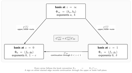
The Gauss hypergeometric equation is the smallest nontrivial global connection problem on the sphere. It has three regular singularities, no accessory parameter, and generic connection coefficients that are explicit gamma quotients. That combination makes it the control experiment for every later Heun, isomonodromic, conformal-block, and exact-WKB connection formula.

The goal here is not merely to quote Euler’s continuation identity. We will fix unit-leading bases, a matrix direction, a continuation path, and branch values; compute the matrices connecting all three singular points; audit their determinants with Wronskians; and turn one matrix entry into the exact Jacobi spectrum. The generic formulas exclude resonance, but the final section explains how to take a resonant basis limit without mistaking a divergent coefficient for a divergent solution.

Three singularities and one normalization ledger

The equation is

$$z(1-z)y'' + \bigl[c-(a+b+1)z\bigr]y' - ab\,y =0.$$

Set

$$\delta=c-a-b.$$

The local exponent pairs are

Point	Exponents	Difference used below
$z=0$	$0,\ 1-c$	$\theta_0=1-c$
$z=1$	$0,\ \delta$	$\theta_1=\delta$
$z=\infty$	$a,\ b$	$\theta_\infty=a-b$

At infinity, exponent $a$ means a solution proportional to $z^{-a}$ in the original coordinate, or to $w^a$ in the local coordinate $w=1/z$. The Fuchs sum is

$$\bigl[0+(1-c)\bigr] + \bigl[0+\delta\bigr] + (a+b) =1.$$

For the generic three-basis calculation assume

$$c\notin\mathbb Z, \qquad \delta\notin\mathbb Z, \qquad a-b\notin\mathbb Z.$$

The first condition is needed for the displayed basis at zero, the second for the basis at one, and the third only when a diagonal Frobenius basis at infinity is used. Thus the zero-to-one calculation itself does not require $a-b\notin\mathbb Z$. These local nonresonance conditions do not forbid a reciprocal gamma factor from vanishing; such a zero will be the spectral mechanism in the Jacobi example.

For the zero-to-one connection, work on

$$\Omega_{01} = \mathbb C \setminus \bigl( (-\infty,0]\cup[1,\infty) \bigr),$$

with $\Log z$ and $\Log(1-z)$ real on $0<z<1$. Continue every local solution to the base point $z_*=1/2$ through that interval. Ordered scalar bases are understood as the columns of the companion fundamental matrix, and the book’s direction remains

$$\Phi_\beta=\Phi_\alpha C_{\alpha\beta}.$$

Unit-leading bases at zero and one

At $z=0$, choose

$$\begin{aligned} f_0(z) &= {}_2F_1 \left( \begin{matrix} a,\ b\\ c \end{matrix} ;z \right),\\ g_0(z) &= z^{1-c} {}_2F_1 \left( \begin{matrix} a-c+1,\ b-c+1\\ 2-c \end{matrix} ;z \right). \end{aligned}$$

Thus

$$f_0(z)=1+O(z), \qquad g_0(z)=z^{1-c}\bigl[1+O(z)\bigr].$$

At $z=1$, the corresponding unit-leading basis is

$$\begin{aligned} f_1(z) &= {}_2F_1 \left( \begin{matrix} a,\ b\\ 1-\delta \end{matrix} ;1-z \right),\\ g_1(z) &= (1-z)^\delta {}_2F_1 \left( \begin{matrix} c-a,\ c-b\\ 1+\delta \end{matrix} ;1-z \right). \end{aligned}$$

In particular,

$$f_1(z)=1+O(1-z), \qquad g_1(z)=(1-z)^\delta\bigl[1+O(1-z)\bigr].$$

The fractional power in the second solution is $(1-z)^\delta$, not $z^\delta$. The distinction is invisible at the level of an exponent table but fatal in a connection calculation.

Write

$$\Phi_0=(f_0,g_0), \qquad \Phi_1=(f_1,g_1).$$

Each column has leading coefficient one in its declared local coordinate. This unit-leading choice is what makes the following gamma matrix a well-defined object rather than a matrix modulo diagonal rescaling.

The zero-to-one gamma matrix

Euler continuation gives

$$\Phi_0=\Phi_1C_{10}, \qquad C_{10} = \begin{pmatrix} A_f&A_g\\ B_f&B_g \end{pmatrix},$$

where

$$\begin{aligned} A_f &= \frac{ \Gamma(c)\Gamma(\delta) }{ \Gamma(c-a)\Gamma(c-b) },& B_f &= \frac{ \Gamma(c)\Gamma(-\delta) }{ \Gamma(a)\Gamma(b) },\\ A_g &= \frac{ \Gamma(2-c)\Gamma(\delta) }{ \Gamma(1-a)\Gamma(1-b) },& B_g &= \frac{ \Gamma(2-c)\Gamma(-\delta) }{ \Gamma(a-c+1)\Gamma(b-c+1) }. \end{aligned}$$

The columns, rather than the rows, carry the two expansions:

$$\begin{aligned} f_0&=A_f f_1+B_f g_1,\\ g_0&=A_g f_1+B_g g_1. \end{aligned}$$

This is the most common place for an unnoticed transpose. A formula written for a vertical vector of scalar functions uses the transpose of the matrix that right-multiplies a fundamental frame.

Two limits explain the first column

When $\operatorname{Re}\delta>0$, the second $z=1$ mode tends to zero. Gauss summation therefore gives

$$\begin{aligned} A_f &= \lim_{z\to1}f_0(z)\\ &= {}_2F_1 \left( \begin{matrix} a,\ b\\ c \end{matrix} ;1 \right)\\ &= \frac{ \Gamma(c)\Gamma(c-a-b) }{ \Gamma(c-a)\Gamma(c-b) }. \end{aligned}$$

For $\operatorname{Re}\delta<0$, use Euler’s transformation

$$f_0(z) = (1-z)^\delta {}_2F_1 \left( \begin{matrix} c-a,\ c-b\\ c \end{matrix} ;z \right).$$

Then a second Gauss sum yields

$$\begin{aligned} B_f &= \lim_{z\to1} (1-z)^{-\delta}f_0(z)\\ &= \frac{ \Gamma(c)\Gamma(a+b-c) }{ \Gamma(a)\Gamma(b) }. \end{aligned}$$

The two half-plane derivations determine meromorphic functions of $a,b,c$, and analytic continuation supplies the generic formula elsewhere. Applying the same argument after the parameter shift

$$(a,b,c) \longmapsto (a-c+1,b-c+1,2-c)$$

gives $A_g$ and $B_g$. Euler’s transformation identifies the resulting local vectors with the already normalized one-basis:

$$\begin{aligned} z^{1-c} {}_2F_1 \left( \begin{matrix} a-c+1,\ b-c+1\\ 1-\delta \end{matrix} ;1-z \right) &= f_1(z),\\ z^{1-c}(1-z)^\delta {}_2F_1 \left( \begin{matrix} 1-a,\ 1-b\\ 1+\delta \end{matrix} ;1-z \right) &= g_1(z). \end{aligned}$$

Wronskians fix the determinant

In monic form, the coefficient of $y'$ is

$$p(z) = \frac{c}{z} + \frac{\delta-1}{1-z}.$$

Abel’s identity, $\Wr'=-p\Wr$, and the unit-leading terms give

$$\begin{aligned} \Wr[f_0,g_0] &= (1-c) z^{-c}(1-z)^{\delta-1},\\ \Wr[f_1,g_1] &= -\delta\, z^{-c}(1-z)^{\delta-1}. \end{aligned}$$

Since $\Phi_0=\Phi_1C_{10}$,

$$\det C_{10} = \frac{\Wr[f_0,g_0]}{\Wr[f_1,g_1]} = \frac{1-c}{-\delta} = \frac{1-c}{a+b-c}.$$

Equivalently, direct gamma simplification first gives

$$\begin{aligned} \det C_{10} ={}& \frac{ \Gamma(c)\Gamma(2-c) \Gamma(\delta)\Gamma(-\delta) }{\pi^2}\\ &\times \Bigl[ \sin\!\bigl(\pi(c-a)\bigr) \sin\!\bigl(\pi(c-b)\bigr)\\ &\qquad - \sin(\pi a)\sin(\pi b) \Bigr]. \end{aligned}$$

The bracket is $\sin(\pi c)\sin(\pi\delta)$. The reflection formula $\Gamma(x)\Gamma(1-x)=\pi/\sin(\pi x)$ then reduces this expression to the Wronskian result. In particular, the four gamma quotients satisfy

$$A_fB_g-A_gB_f = \frac{1-c}{-\delta}.$$

The Wronskian proof explains why this identity had to be true. It also catches a reversed matrix direction: taking the inverse would invert the determinant.

The reverse connection is

$$\begin{aligned} C_{01} = C_{10}^{-1} = \frac{-\delta}{1-c} \begin{pmatrix} B_g&-A_g\\ -B_f&A_f \end{pmatrix}. \end{aligned}$$

Infinity remembers the continuation path

Connections to infinity require one more datum: whether the base interval is left through the upper or lower half-plane. Choose $R>1$ and normalize the infinity powers by taking $\Log R$ real. The fixed unit-leading basis is

$$\begin{aligned} h_a(z) &= z^{-a} {}_2F_1 \left( \begin{matrix} a,\ a-c+1\\ a-b+1 \end{matrix} ;\frac1z \right),\\ h_b(z) &= z^{-b} {}_2F_1 \left( \begin{matrix} b,\ b-c+1\\ b-a+1 \end{matrix} ;\frac1z \right). \end{aligned}$$

Let $\gamma_s$ continue from $z_*=1/2$ to $R$, where $s=+1$ labels the upper path around one and $s=-1$ the lower path. At the endpoint,

$$\arg(1-z)=-s\pi, \qquad \arg(-z)=-s\pi.$$

Consequently,

$$\begin{aligned} (-z)^{-\mu} &= \ee^{s\pi\ii\mu}z^{-\mu},\\ (1-z)^\delta &= \ee^{-s\pi\ii\delta}(z-1)^\delta. \end{aligned}$$

This phase ledger determines every lateral factor. With $\Phi_\infty=(h_a,h_b)$, the path-labelled connection is

$$\Phi_0 = \Phi_\infty C_{\infty0}^{(s)}, \qquad C_{\infty0}^{(s)} = \begin{pmatrix} \ee^{s\pi\ii a}P_a & \ee^{s\pi\ii(a-c+1)}Q_a\\ \ee^{s\pi\ii b}P_b & \ee^{s\pi\ii(b-c+1)}Q_b \end{pmatrix},$$

where

$$\begin{aligned} P_a &= \frac{ \Gamma(c)\Gamma(b-a) }{ \Gamma(b)\Gamma(c-a) },& P_b &= \frac{ \Gamma(c)\Gamma(a-b) }{ \Gamma(a)\Gamma(c-b) },\\ Q_a &= \frac{ \Gamma(2-c)\Gamma(b-a) }{ \Gamma(b-c+1)\Gamma(1-a) },& Q_b &= \frac{ \Gamma(2-c)\Gamma(a-b) }{ \Gamma(a-c+1)\Gamma(1-b) }. \end{aligned}$$

The first column contains the lateral values of $(-z)^{-a}$ and $(-z)^{-b}$. In the second column, the prefactor $z^{1-c}$ shifts those phases by $\ee^{s\pi\ii(1-c)}$. Suppressing either contribution silently changes the normalization of the infinity basis.

The determinant has two equivalent audits:

$$\begin{aligned} \det C_{\infty0}^{(s)} &= \ee^{s\pi\ii(1-\delta)} \bigl(P_aQ_b-Q_aP_b\bigr)\\ &= \frac{1-c}{a-b} \ee^{s\pi\ii(1-\delta)}. \end{aligned}$$

For the fixed infinity basis,

$$\Wr[h_a,h_b] = (a-b) z^{-c}(z-1)^{\delta-1}.$$

Since

$$(1-z)^{\delta-1} = \ee^{s\pi\ii(1-\delta)} (z-1)^{\delta-1}$$

along $\gamma_s$, the Wronskian ratio reproduces the same result.

The directed connection triangle. Matrix subscripts follow $\Phi_\beta=\Phi_\alpha C_{\alpha\beta}$, and the sign labels the continuation path whenever infinity is involved.

The third edge can be written without a new derivation. The connection cocycle gives

$$C_{\infty0}^{(s)} = C_{\infty1}^{(s)}C_{10},$$

where

$$\begin{aligned} C_{\infty1}^{(s)} &= \begin{pmatrix} U_a&\ee^{-s\pi\ii\delta}V_a\\ U_b&\ee^{-s\pi\ii\delta}V_b \end{pmatrix},\\ U_a &= \frac{ \Gamma(1-\delta)\Gamma(b-a) }{ \Gamma(b)\Gamma(b-c+1) },\\ U_b &= \frac{ \Gamma(1-\delta)\Gamma(a-b) }{ \Gamma(a)\Gamma(a-c+1) },\\ V_a &= \frac{ \Gamma(1+\delta)\Gamma(b-a) }{ \Gamma(c-a)\Gamma(1-a) },\\ V_b &= \frac{ \Gamma(1+\delta)\Gamma(a-b) }{ \Gamma(c-b)\Gamma(1-b) }. \end{aligned}$$

Its determinant supplies a compact cocycle audit:

$$\det C_{\infty1}^{(s)} = \frac{\delta}{a-b} \ee^{-s\pi\ii\delta}, \qquad \det C_{\infty0}^{(s)} = \det C_{\infty1}^{(s)}\det C_{10}.$$

Changing the continuation side changes both the stem and the phases. In terms of the local monodromy matrices introduced next,

$$\begin{aligned} C_{\infty0}^{(+)} &= D_\infty C_{\infty0}^{(-)}D_0,\\ C_{\infty1}^{(+)} &= C_{\infty1}^{(-)}D_1^{-1}. \end{aligned}$$

These relations are useful numerical checks because they test the gamma quotients, branch factors, and basis ordering at once.

For the reproducible sample

$$a=\frac13, \qquad b=\frac25, \qquad c=\frac76, \qquad \delta=\frac{13}{30},$$

the upper-route determinants are

$$\begin{aligned} \det C_{10} &= \frac5{13},\\ \det C_{\infty0}^{(+)} &= \frac52\ee^{17\pi\ii/30},\\ \det C_{\infty1}^{(+)} &= -\frac{13}{2}\ee^{-13\pi\ii/30}. \end{aligned}$$

Their product has the correct minus-sign phase shift, $-\ee^{-13\pi\ii/30}=\ee^{17\pi\ii/30}$.

Monodromy from diagonal local data

In their own unit-leading bases, positively oriented local loops have diagonal matrices

$$\begin{aligned} D_0 &= \operatorname{diag} \left( 1,\ee^{2\pi\ii(1-c)} \right),\\ D_1 &= \operatorname{diag} \left( 1,\ee^{2\pi\ii\delta} \right),\\ D_\infty &= \operatorname{diag} \left( \ee^{2\pi\ii a}, \ee^{2\pi\ii b} \right). \end{aligned}$$

For $D_\infty$, “positive” refers to the local coordinate $w=1/z$; in the $z$-plane it is a clockwise large circle. Transporting to the $z=0$ frame with the lower stem gives

$$\begin{aligned} M_0^{(0)} &=D_0,\\ M_1^{(0)} &=C_{10}^{-1}D_1C_{10},\\ M_\infty^{(0)} &= \left( C_{\infty0}^{(-)} \right)^{-1} D_\infty C_{\infty0}^{(-)}. \end{aligned}$$

Choose the distinguished based loops in the order fixed on the monodromy page. In the book’s composition convention, the rightmost loop is traversed first; the matrix farther left belongs to the path traversed later. Then

$$M_0^{(0)}M_1^{(0)}M_\infty^{(0)}=I.$$

The determinant of this relation already follows from the Fuchs sum:

$$\begin{aligned} \det D_0\det D_1\det D_\infty &= \exp\left\{ 2\pi\ii \bigl[ (1-c)+\delta+a+b \bigr] \right\}\\ &= \ee^{2\pi\ii}=1. \end{aligned}$$

The full matrix relation additionally tests the continuation paths and connection directions. An upper stem gives a different distinguished loop system; with its corresponding infinity matrix, the order is $M_1^{(0)}M_0^{(0)}M_\infty^{(+)}=I$. A lateral phase cannot be changed while keeping the based-loop word fixed.

This three-puncture system is rigid in the generic irreducible case: once the local conjugacy classes and marking are fixed, the monodromy tuple is determined up to simultaneous conjugacy. There is no accessory parameter to vary. The gamma matrix is therefore not one possible answer among a continuous family. It is the normalization-complete realization of the rigid connection problem. The four-singularity Heun equation loses this simplicity because an accessory parameter remains.

Local nonresonance is not the same as global irreducibility. The Gauss monodromy representation is irreducible precisely when none of

$$a,\qquad b,\qquad c-a,\qquad c-b$$

is an integer. The gamma entries make the reducible loci visible, while $c$, $\delta$, and $a-b$ govern whether the displayed local bases are resonant.

A Jacobi spectrum from one reciprocal-gamma factor

Let $\alpha,\beta>-1$ and work in

$$L^2\!\left( (0,1); z^\alpha(1-z)^\beta\,\dd z \right).$$

Consider the weighted problem

$$\begin{aligned} - \frac{1}{ z^\alpha(1-z)^\beta } \frac{\dd}{\dd z} \left[ z^{\alpha+1}(1-z)^{\beta+1}y' \right] = \lambda y \end{aligned}$$

on $0<z<1$. Select the endpoint-regular Jacobi realization: at each regular or limit-circle endpoint impose the separated flux condition

$$\lim_{z\to0^+} z^{\alpha+1}(1-z)^{\beta+1}y'(z) =0, \qquad \lim_{z\to1^-} z^{\alpha+1}(1-z)^{\beta+1}y'(z) =0.$$

At zero, the endpoint is regular for $-1<\alpha<0$, singular limit-circle for $0\leq\alpha<1$, and limit-point for $\alpha\geq1$. Replace $\alpha$ by $\beta$ for the endpoint at one. No condition is imposed at a limit-point endpoint; square integrability selects the analytic branch there. Thus, for nonintegral $\alpha,\beta$, the stated domain selects the analytic Frobenius branch at each end. The expanded equation is hypergeometric with

$$\begin{aligned} c&=\alpha+1,\\ a+b&=\alpha+\beta+1,\\ ab&=-\lambda,\\ \delta&=-\beta. \end{aligned}$$

Assume first that $\alpha$ and $\beta$ are nonintegral so the generic bases apply. The solution analytic at zero is $f_0$. Near one,

$$f_0=A_f f_1+B_f g_1,$$

and $g_1$ carries the nonanalytic exponent $-\beta$. The right endpoint condition is therefore

$$B_f(\lambda) = \frac{ \Gamma(\alpha+1)\Gamma(\beta) }{ \Gamma(a)\Gamma(b) } =0.$$

The gamma function has no zeros, while $1/\Gamma$ vanishes at the nonpositive integers. Hence

$$a=-n \quad\text{or}\quad b=-n, \qquad n\in\mathbb Z_{\ge0}.$$

Using $a+b=\alpha+\beta+1$ gives

$$\lambda_n = n(n+\alpha+\beta+1).$$

For $a=-n$,

$$\begin{aligned} y_n(z) &= {}_2F_1 \left( \begin{matrix} -n,\ n+\alpha+\beta+1\\ \alpha+1 \end{matrix} ;z \right)\\ &= \frac{n!}{(\alpha+1)_n} P_n^{(\alpha,\beta)}(1-2z). \end{aligned}$$

Thus polynomial truncation, a boundary-function zero, and the Sturm–Liouville spectrum are the same event in three languages. Integral $\alpha$ or $\beta$ requires a resonant local basis, but the spectrum and Jacobi polynomial follow by a controlled parameter limit. Other self-adjoint endpoint conditions in limit-circle cases are different spectral problems and need not select the same connection entry.

The coefficient $B_f$ is a normalized spectral boundary function. Its zeros are intrinsic under nonvanishing analytic rescalings, but it is not automatically a Fredholm or zeta determinant; the distinctions are explained on the boundary-functions page.

Resonance is a basis limit, not direct substitution

When $c\in\mathbb Z$, $\delta\in\mathbb Z$, or $a-b\in\mathbb Z$, one local exponent difference is integral. A logarithmic solution may appear, and the corresponding pair above ceases to be an invertible unit-leading frame. Gamma factors that diverge in $C_{10}$ are then warning about the degenerating basis, not automatically about the analytically continued solution.

For example, hold $a,b$ fixed and set $c=a+b+\varepsilon$, so $\delta=\varepsilon\to0$. The two $z=1$ modes coalesce. Before taking the limit, replace them by

$$\begin{aligned} u_1(\varepsilon) &= f_1(\varepsilon),\\ v_1(\varepsilon) &= \frac{ g_1(\varepsilon)-f_1(\varepsilon) }{ \varepsilon }. \end{aligned}$$

Then

$$\Phi_1(\varepsilon) = \bigl( u_1(\varepsilon), v_1(\varepsilon) \bigr) \begin{pmatrix} 1&1\\ 0&\varepsilon \end{pmatrix}.$$

If

$$S(\varepsilon) = \begin{pmatrix} 1&1\\ 0&\varepsilon \end{pmatrix},$$

then $\Phi_1=\widehat\Phi_1S$ and

$$\Phi_0 = \widehat\Phi_1\widehat C_{10}, \qquad \widehat C_{10} = S C_{10}.$$

Thus the basis-change matrix left-multiplies the singular gamma matrix before $\varepsilon\to0$; its divergent pieces cancel. The limiting $v_1$ contains the expected $\log(1-z)$ term. Consistently, the zero-balanced solution has the leading expansion

$$\begin{aligned} {}_2F_1(a,b;a+b;z) ={}& \frac{\Gamma(a+b)}{\Gamma(a)\Gamma(b)} \Bigl[ -\log(1-z)\\ &\quad +2\psi(1)-\psi(a)-\psi(b) \Bigr]\\ &+ O\!\bigl((1-z)\log(1-z)\bigr). \end{aligned}$$

The same workflow applies at zero or infinity:

1. move off resonance;
2. choose combinations that converge to a Frobenius–logarithmic basis;
3. transform the connection matrix;
4. take the parameter limit;
5. recheck the limiting Wronskian and monodromy Jordan form.

Kummer’s 24 named solutions do not provide 24 independent functions. They are transformed presentations of the same two-dimensional solution space, and at resonance some presentations coalesce.

For a numerical gamma-matrix checkpoint away from resonance, see the Gauss connection example.

Common pitfalls

Using the wrong local power at one. The second $z=1$ mode begins with $(1-z)^\delta$. Replacing it by $z^\delta$ destroys the local exponent and invalidates every coefficient that follows.

Transposing without noticing. A vertical vector of scalar solutions and a right-acting fundamental frame use transposed coefficient arrays. Test the first column against $f_0=A_f f_1+B_f g_1$.

Dropping the route to infinity. The upper and lower matrices contain different exponent-dependent phases in every row. Their exact change is controlled by $D_\infty C_{\infty0}^{(-)}D_0$, so it is monodromy, not a cosmetic convention.

Reading a gamma pole as a physical divergence. At resonance, the local basis is singular. Recombine the basis before taking the limit.

Confusing a coefficient zero with a gamma zero. Gamma has no zeros. Hypergeometric quantization comes from a pole in a denominator gamma function, equivalently a zero of its reciprocal.

Exercises

1. Recover the exponent ledger. Derive the indicial exponents at $0$, $1$, and infinity, and verify the Fuchs sum.

Solution

At zero, substitute $y=z^\rho$ and keep the coefficient of $z^{\rho-1}$:

$$\rho(\rho-1)+c\rho = \rho(\rho+c-1)=0.$$

Thus $\rho=0,1-c$. With $t=1-z$, the same calculation gives

$$\rho(\rho-\delta)=0,$$

so the exponents at one are $0,\delta$. At infinity, set $w=1/z$ and $y=z^{-\rho}$; the leading equation gives

$$(\rho-a)(\rho-b)=0.$$

Therefore

$$(1-c)+\delta+a+b=1.$$

2. Derive the second column. Apply the first-column argument to $g_0$ after shifting $(a,b,c)\mapsto(a-c+1,b-c+1,2-c)$. Recover $A_g$ and $B_g$.

Solution

The shifted exponent difference at one is still

$$(2-c)-(a-c+1)-(b-c+1)=\delta.$$

Gauss summation gives the coefficient of the exponent-zero mode:

$$A_g = \frac{ \Gamma(2-c)\Gamma(\delta) }{ \Gamma(1-a)\Gamma(1-b) }.$$

Euler transformation followed by the second Gauss sum gives

$$B_g = \frac{ \Gamma(2-c)\Gamma(-\delta) }{ \Gamma(a-c+1)\Gamma(b-c+1) }.$$

Euler’s transformation gives the two exact basis-identification identities displayed in the main derivation. The factor $z^{1-c}$ is unit-valued at $z=1$ on the declared branch, so no additional zero-to-one phase remains.

3. Audit the gamma determinant. Starting from the four gamma quotients, show directly that

$$A_fB_g-A_gB_f = \frac{1-c}{-\delta}.$$

Solution

Factor out

$$\Gamma(c)\Gamma(2-c)\Gamma(\delta)\Gamma(-\delta).$$

Use

$$\Gamma(x)\Gamma(1-x) = \frac{\pi}{\sin(\pi x)}$$

on each complementary denominator pair. This gives

$$\begin{aligned} \det C_{10} ={}& \frac{ \Gamma(c)\Gamma(2-c) \Gamma(\delta)\Gamma(-\delta) }{\pi^2}\\ &\times \Bigl[ \sin\!\bigl(\pi(c-a)\bigr) \sin\!\bigl(\pi(c-b)\bigr)\\ &\qquad - \sin(\pi a)\sin(\pi b) \Bigr]. \end{aligned}$$

Since $c=a+b+\delta$, the bracket equals $\sin(\pi c)\sin(\pi\delta)$. Applying reflection once more yields

$$\frac{1-c}{-\delta}.$$

The Wronskian computation in the text is a shorter proof and fixes the sign without trigonometric bookkeeping.

4. Reverse the connection. Verify the displayed formula for $C_{01}$, and write $f_1$ and $g_1$ explicitly in the zero basis.

Solution

For a two-by-two matrix,

$$C_{10}^{-1} = \frac1{\det C_{10}} \begin{pmatrix} B_g&-A_g\\ -B_f&A_f \end{pmatrix}.$$

Since $\det C_{10}=(1-c)/(-\delta)$,

$$C_{01} = \frac{-\delta}{1-c} \begin{pmatrix} B_g&-A_g\\ -B_f&A_f \end{pmatrix}.$$

The columns of $\Phi_1=\Phi_0C_{01}$ therefore give

$$\begin{aligned} f_1 &= \frac{-\delta}{1-c} \bigl(B_gf_0-B_fg_0\bigr),\\ g_1 &= \frac{-\delta}{1-c} \bigl(-A_gf_0+A_fg_0\bigr). \end{aligned}$$

5. Recover the infinity phases. With $z^{-a}$ and $z^{-b}$ positive at $R>1$, derive the two columns of $C_{\infty0}^{(s)}$ and prove

$$\det C_{\infty0}^{(s)} = \frac{1-c}{a-b}\ee^{s\pi\ii(1-\delta)}.$$

Solution

At $R>1$ reached along $\gamma_s$,

$$\arg(-z)=-s\pi, \qquad \arg(1-z)=-s\pi.$$

Hence the first-column infinity powers contribute $\ee^{s\pi\ii a}$ and $\ee^{s\pi\ii b}$. For the shifted first term in $g_0$,

$$z^{1-c}(-z)^{-(a-c+1)} = \ee^{s\pi\ii(a-c+1)}z^{-a},$$

and similarly for the $b$ row. Direct gamma simplification gives

$$P_aQ_b-Q_aP_b = \frac{1-c}{a-b}.$$

Both determinant terms carry the common phase $\ee^{s\pi\ii(a+b-c+1)} =\ee^{s\pi\ii(1-\delta)}$, which proves the result.

6. Transport local monodromy. Prove that $M_1^{(0)}$ has the same eigenvalues and determinant as $D_1$, and verify the determinant part of $M_0^{(0)}M_1^{(0)}M_\infty^{(0)}=I$ for the lower stem.

Solution

Similarity preserves the characteristic polynomial, so

$$M_1^{(0)} = C_{10}^{-1}D_1C_{10}$$

has eigenvalues $1,\ee^{2\pi\ii\delta}$ and determinant $\ee^{2\pi\ii\delta}$. Multiplying all three local determinants gives

$$\begin{aligned} \det M_0^{(0)} \det M_1^{(0)} \det M_\infty^{(0)} &= \ee^{2\pi\ii[(1-c)+\delta+a+b]}\\ &= \ee^{2\pi\ii}=1. \end{aligned}$$

This checks the scalar determinant relation. The full matrix identity also depends on the compatible based-loop tails.

7. Derive Jacobi quantization. Starting from $B_f=0$, derive $\lambda_n$ and the normalized Jacobi-polynomial solution.

Solution

The right endpoint coefficient is

$$B_f = \frac{ \Gamma(\alpha+1)\Gamma(\beta) }{ \Gamma(a)\Gamma(b) }.$$

In the nonresonant calculation its zero requires $a=-n$ or $b=-n$. Choose $a=-n$. Since $a+b=\alpha+\beta+1$,

$$b=n+\alpha+\beta+1.$$

Using $ab=-\lambda$ gives

$$\lambda_n=n(n+\alpha+\beta+1).$$

Finally, the standard hypergeometric representation of the Jacobi polynomial is

$$P_n^{(\alpha,\beta)}(1-2z) = \frac{(\alpha+1)_n}{n!} {}_2F_1 \left( \begin{matrix} -n,\ n+\alpha+\beta+1\\ \alpha+1 \end{matrix} ;z \right),$$

which yields the normalization stated in the text.

8. Build the zero-balanced logarithmic mode. Hold $a,b$ fixed and set $c=a+b+\varepsilon$. Show from the leading local factors that

$$v_1(\varepsilon) = \frac{g_1(\varepsilon)-f_1(\varepsilon)}{\varepsilon}$$

has a finite limit whose leading logarithmic term is $\log(1-z)$.

Solution

Put $t=1-z$ and write

$$\begin{aligned} f_1(\varepsilon) &= {}_2F_1(a,b;1-\varepsilon;t),\\ g_1(\varepsilon) &= t^\varepsilon {}_2F_1 \left( \begin{matrix} b+\varepsilon,\ a+\varepsilon\\ 1+\varepsilon \end{matrix} ;t \right). \end{aligned}$$

At $\varepsilon=0$, both series equal $F(t)={}_2F_1(a,b;1;t)$. Differentiate the analytic parameter dependence of the two series and use $t^\varepsilon=1+\varepsilon\Log t+O(\varepsilon^2)$. The quotient tends to

$$\lim_{\varepsilon\to0} v_1(\varepsilon) = F(t)\Log t + H(t),$$

where $H$ is holomorphic near zero. Thus the leading term is $\Log(1-z)$, while higher powers of $1-z$ can also multiply the logarithm. Parameter derivatives of the hypergeometric series contribute to $H$. Transforming the connection matrix before taking the limit cancels its $1/\varepsilon$ gamma poles.

References

• NIST Digital Library of Mathematical Functions, 15.10.1 for the Gauss equation, 15.11.4 for its Riemann scheme, and 15.11.2 for the Fuchs exponent sum.
• NIST Digital Library of Mathematical Functions, §15.10, Hypergeometric Differential Equation, especially 15.10.2–7 for the three local bases and Wronskians, and 15.10.17–28 for principal-branch connection formulas.
• NIST Digital Library of Mathematical Functions, 15.4.20 for Gauss summation, 15.8.1 for Euler–Pfaff transformations, 15.8.2 for inverse-variable continuation, and 15.8.8–11 for resonant limits.
• NIST Digital Library of Mathematical Functions, 1.13.4–5 for the Wronskian convention and Abel’s identity, and 2.7.6 for the Frobenius–logarithmic form.
• NIST Digital Library of Mathematical Functions, §18.5, Explicit Representations, for the hypergeometric representation of Jacobi polynomials.
• NIST Digital Library of Mathematical Functions, §5.2(i), Gamma and Psi Functions, for the poles and absence of zeros of $\Gamma$, and the zeros of $1/\Gamma$.
• G. E. Andrews, R. Askey, and R. Roy, Special Functions, Cambridge University Press, 1999, Chapter 2, for Gauss summation, transformations, and the hypergeometric differential equation.
• A. Erdélyi, W. Magnus, F. Oberhettinger, and F. G. Tricomi, Higher Transcendental Functions, volume I, McGraw–Hill, 1953, Chapter II, especially §2.9 for the instruction to reverse exponential signs on lower-half-plane continuation.
• K. Iwasaki, H. Kimura, S. Shimomura, and M. Yoshida, From Gauss to Painlevé: A Modern Theory of Special Functions, Vieweg, 1991, for hypergeometric monodromy, rigidity, and its role in the passage to Painlevé equations.
• F. Beukers and G. Heckman, “Monodromy for the Hypergeometric Function ${}_nF_{n-1}$”, Inventiones Mathematicae 95 (1989), 325–354, especially Propositions 2.7 and 3.2–3.3 and Theorem 3.5 for reducibility, irreducibility, and rigidity.
• G. Szegő, Orthogonal Polynomials, American Mathematical Society, fourth edition, 1975, for classical Jacobi polynomial theory.
• F. Gesztesy, L. L. Littlejohn, M. Piorkowski, and J. Stanfill, “The Jacobi Operator on $(-1,1)$ and Its Various $m$-Functions”, Complex Analysis and Operator Theory 18, 155 (2024), for endpoint classification and self-adjoint realizations selecting Jacobi polynomials.
• N. M. Katz, Rigid Local Systems, Princeton University Press, 1996, for the general rigidity framework.