Analytic Classification and Sectorial Normalization

A formal normal form identifies the exponential scales near an irregular singularity, but its normalizing series usually diverges. The analytic problem is to realize that series by genuine solutions on sectors and then measure how neighboring realizations disagree.

The disagreement is exponentially small, constant in a solution basis, and recorded by Stokes matrices. Together with the formal type, these matrices are the missing local analytic invariants. This page makes that statement precise, fixes all crossing and product conventions, and computes one nontrivial multiplier from first principles.

Two phase conditions, two different roles

For an exponential difference $\Delta q$, the condition $\operatorname{Re}\Delta q=0$ marks equal magnitude. A singular Borel–Laplace direction instead occurs when a relevant exponential is maximally decaying. Because the names “Stokes” and “anti-Stokes” are reversed in parts of the literature, this book always states the phase condition.

Sectors and asymptotic meaning

Work in the coordinate in which the formal decomposition is unramified. If the original coordinate is $x$ and the minimal cover is $x=t^p$, all angular statements in this section refer to the $t$-plane. On its universal cover, write

$$S(a,b;\rho) = \left\{ 0<|t|<\rho,\; a<\arg t<b \right\}.$$

A proper closed subsector is obtained by shrinking the radius and moving both boundary angles strictly inward. An analytic matrix $H(t)$ has the Poincaré expansion

$$H(t)\sim\widehat H(t) =\sum_{n=0}^{\infty}H_nt^n$$

on $S$ when, on every proper closed subsector and for every $N\geq0$,

$$\left\| H(t)-\sum_{n=0}^{N-1}H_nt^n \right\| \leq C_N|t|^N.$$

This definition is local in angle as well as radius. It does not assert that the series converges, and it does not make its analytic realization unique. For example, if

$$\operatorname{Re}\left(\frac{c}{t^k}\right)>0,$$

then $\exp(-c/t^k)$ is smaller than every power of $t$ on proper closed subsectors. Adding it changes the function without changing its Poincaré series.

The expansion is Gevrey-$1/k$ if the remainder has the stronger estimate

$$\left\| H(t)-\sum_{n=0}^{N-1}H_nt^n \right\| \leq CA^N\Gamma\left(1+\frac{N}{k}\right)|t|^N$$

for suitable $C,A>0$, locally uniformly in angle. At one level $k$, Watson uniqueness requires an opening strictly greater than $\pi/k$. Equality is not enough: a function such as $\exp(-c/t^k)$ can remain flat on every proper closed subsector of a sector of opening $\pi/k$.

From a formal gauge to canonical sectorial solutions

After formal reduction on $x=t^p$, write schematically

$$\widehat\Phi(t) = \widehat H(t)F(t), \qquad F(t) = \operatorname{diag}_{\alpha} \left( \ee^{q_\alpha(t)}t^{L_\alpha} \right).$$

The diagonal notation suppresses regular-singular blocks; repeated exponential factors must be kept together. The formal matrix $\widehat H$ is invertible in formal power series, while each $q_\alpha$ is a finite polynomial in $t^{-1}$ without constant term.

The sectorial normalization theorem supplies analytic invertible matrices $H_j$ on a suitable covering by sectors such that

$$H_j\sim\widehat H, \qquad \Phi_j=H_jF$$

is an exact fundamental matrix. For a single positive level $k$, $\widehat H$ is $k$-summable away from finitely many singular directions, and its directional sums provide the $H_j$. When several degrees occur among the differences $q_\alpha-q_\beta$, one generally needs multisummation, with the levels treated in their prescribed order.

The theorem does not select a basis from the equation alone. A canonical sectorial basis also requires:

• an ordering and normalization of the formal blocks;
• a branch of $\operatorname{Log}t$ and, when present, a deck identification;
• the sectors and their counterclockwise indexing;
• a lateral prescription on a singular direction.

Once these choices are fixed, exponentially small ambiguities become well-defined matrices rather than informal correction terms.

Dominance geometry and singular directions

For an ordered pair of formal blocks, suppose

$$\Delta q_{\alpha\beta}(t) =q_\alpha(t)-q_\beta(t) =c_{\alpha\beta}t^{-k} +O(t^{-k+1}), \qquad c_{\alpha\beta}\neq0.$$

Along $t=r\ee^{\ii\theta}$,

$$\operatorname{Re}\Delta q_{\alpha\beta} \sim r^{-k} \operatorname{Re} \left( c_{\alpha\beta}\ee^{-\ii k\theta} \right).$$

There are three distinct statements:

Phase condition	Meaning
$\operatorname{Re}\Delta q_{\alpha\beta}>0$	The $\alpha$ exponential dominates the $\beta$ exponential
$\operatorname{Re}\Delta q_{\alpha\beta}=0$	The two exponentials have equal leading magnitude
$c_{\alpha\beta}\ee^{-\ii k\theta}\in\mathbb R_{<0}$	$\ee^{\Delta q_{\alpha\beta}}$ is maximally decaying; this is the ordered-pair singular or jump direction used here

The last condition is also where the corresponding Borel singularity can obstruct directional Laplace summation. Reversing the ordered pair replaces $c_{\alpha\beta}$ by $-c_{\alpha\beta}$ and changes the relevant direction.

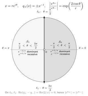
Dominance sectors for $q_\pm(x)=\pm x^{-1}$. The marked rays satisfy $\operatorname{Re}(q_+-q_-)=0$ and exchange the dominant exponential. They are equal-magnitude directions; terminology in the literature varies. The geometry alone does not imply a nonzero Stokes multiplier.

For this figure, $q_+-q_-=2/x$. Equal magnitude occurs at $\arg x=\pm\pi/2$. The ordered-pair singular direction on which $\exp(q_+-q_-)$ is maximally small is instead $\arg x=\pi$; for the reverse ordered pair it is $\arg x=0$.

Stokes matrices from overlapping normalizations

Index the sectorial fundamental matrices counterclockwise and use the book’s right-action convention

$$\Phi_{j+1}=\Phi_jS_j$$

on a connected overlap. The transition is constant because

$$\frac{\dd}{\dd t} \left( \Phi_j^{-1}\Phi_{j+1} \right) =0.$$

After the formal block normalization is fixed, $S_j$ is unipotent and lies in the Stokes group allowed by the dominance ordering on that overlap. Its off-diagonal entries are the Stokes multipliers.

In a generic rank-two, one-level problem, suppose $\exp(q_1-q_2)$ is flat on the overlap. Then the first column is subdominant relative to the second, and the allowed right factor has the form

$$S_j=I+s_jE_{12}.$$

Indeed, right multiplication adds $s_j$ times column $1$ to column $2$, which does not alter the prescribed power-series asymptotics of the latter. If $\exp(q_2-q_1)$ is flat, the corresponding factor is $I+s_jE_{21}$.

This triangular rule should not be extrapolated blindly. Repeated blocks, several exponential levels, and higher rank replace a total ordering by filtered block Stokes groups. At several levels, the factorization order is part of the data.

Formal periodicity and actual monodromy

Let one positive circuit in the original $x$-plane cross $m$ indexed boundaries. On the universal cover, choose the equivariant normalization

$$\Phi_{j+m}=\Phi_jM_{\mathrm f},$$

where $M_{\mathrm f}$ is the generalized formal monodromy. It includes any deck permutation caused by $x=t^p$, as well as the power-factor action. The transition matrices then obey

$$S_{j+m} =M_{\mathrm f}^{-1}S_jM_{\mathrm f}.$$

The inverse transitions in the actual monodromy product are easy to miss. When a fixed solution basis is continued from sector $j$ to sector $j+1$, the identity

$$\Phi_j=\Phi_{j+1}S_j^{-1}$$

expresses that continued basis in the next canonical basis. After all $m$ crossings,

$$\begin{aligned} \Phi_0^\gamma &= \Phi_m S_{m-1}^{-1}\cdots S_0^{-1}\\ &= \Phi_0 M_{\mathrm f} S_{m-1}^{-1}\cdots S_0^{-1}. \end{aligned}$$

Therefore, with positive continuation acting on the right,

$$M_\gamma = M_{\mathrm f} S_{m-1}^{-1}\cdots S_0^{-1}.$$

Changing the crossing convention to $\Phi_j=\Phi_{j+1}\widetilde S_j$ replaces every factor by its inverse and changes the displayed product. Formulas from two sources cannot be compared until this ledger is translated.

What the analytic classification remembers

The formal type records the ramification, exponential factors, regular-singular blocks, and formal monodromy. It does not determine the $S_j$. Two meromorphic connections with the same formal type are locally analytically equivalent precisely when their Stokes cocycles agree up to the admissible automorphisms of that formal type. Thus the analytic moduli are, schematically,

$$\left\{ \text{formal type}; \ S_0,\ldots,S_{m-1} \right\} \big/ \left\{ \text{admissible basis changes} \right\}.$$

The quotient is essential. Under one common constant right basis change $C$,

$$\begin{aligned} S_j&\longmapsto C^{-1}S_jC,\\ M_{\mathrm f}&\longmapsto C^{-1}M_{\mathrm f}C,\\ M_\gamma&\longmapsto C^{-1}M_\gamma C. \end{aligned}$$

More generally, sector-dependent changes $\widetilde\Phi_j=\Phi_jC_j$ give

$$\widetilde S_j =C_j^{-1}S_jC_{j+1}.$$

A common single-valued left gauge $\widetilde\Phi_j=G\Phi_j$ leaves the right transition matrices numerically unchanged. For a diagonal rescaling $D=\operatorname{diag}(d_1,\ldots,d_n)$,

$$D^{-1}E_{ij}D =\frac{d_j}{d_i}E_{ij},$$

so an individual multiplier is not basis invariant. Its normalized value, the Stokes conjugacy data, and products entering actual monodromy are the meaningful objects.

A residue computes a Stokes multiplier

Return to the triangular system from formal irregular classification:

$$Y' = \begin{pmatrix} -x^{-2}&x^{-1}\\ 0&0 \end{pmatrix}Y.$$

Its formal fundamental matrix is

$$\widehat\Phi = \begin{pmatrix} 1&\widehat h\\ 0&1 \end{pmatrix} \begin{pmatrix} \ee^{1/x}&0\\ 0&1 \end{pmatrix},$$

where

$$\widehat h(x) = \sum_{n=1}^{\infty} (-1)^{n-1}(n-1)!x^n.$$

Use the order-one Borel transform

$$\mathcal B(x^n) = \frac{\xi^{n-1}}{\Gamma(n)}.$$

It turns the divergent series into the rational germ

$$\mathcal B\widehat h(\xi) = \frac{1}{1+\xi}.$$

Its only finite singularity is $\xi=-1$. Away from the Laplace direction $\theta=\pi$, define

$$h_\theta(x) = \int_0^{\ee^{\ii\theta}\infty} \frac{\ee^{-\xi/x}}{1+\xi}\,\dd\xi, \qquad |\arg x-\theta|<\frac{\pi}{2}.$$

Termwise Laplace integration recovers $\widehat h$. With the lateral convention $\operatorname{Disc}_\pi=h_{\pi+}-h_{\pi-}$, a small contour around the pole gives

$$h_{\pi+}-h_{\pi-} =-2\pi\ii\,\ee^{1/x}.$$

Consequently,

$$\Phi_{\pi+} = \Phi_{\pi-} \left( I-2\pi\ii E_{12} \right).$$

The nonidentity Stokes factor is therefore

$$S=I-2\pi\ii E_{12}.$$

This is a genuine analytic invariant: no finite truncation of $\widehat h$ can see its multiplier.

The same sectorial sum can be written

$$h(x) =-\ee^{1/x}\operatorname{Ei}(-1/x)$$

on a compatible branch. Positive continuation of $x$ decreases the logarithm inside $\operatorname{Ei}(-1/x)$ by $2\pi\ii$, hence

$$h^\gamma=h+2\pi\ii\,\ee^{1/x}.$$

Here $M_{\mathrm f}=I$, the other Stokes factor is the identity, and direct continuation gives

$$M_0=I+2\pi\ii E_{12}=S^{-1},$$

exactly as required by the ordered monodromy product.

A parameter limit turns a jump into a logarithm

Now insert a complex parameter:

$$Y' = \begin{pmatrix} -\lambda x^{-2}&x^{-1}\\ 0&0 \end{pmatrix}Y.$$

For $\lambda\neq0$, the normalizing entry solves

$$x^2h'+\lambda h=x$$

and has formal expansion

$$\widehat h_\lambda(x) = \sum_{n=1}^{\infty} (-1)^{n-1}(n-1)! \left(\frac{x}{\lambda}\right)^n.$$

Its Borel transform is $(\lambda+\xi)^{-1}$. Thus the singular summation direction rotates with the pole $\xi=-\lambda$:

$$\arg x = \arg\lambda-\pi \pmod{2\pi}.$$

The exact branch

$$h_\lambda(x) =-\ee^{\lambda/x} \operatorname{Ei}(-\lambda/x)$$

has the same lateral jump $-2\pi\ii\ee^{\lambda/x}$. Hence the normalized Stokes multiplier and the actual monodromy

$$S_\lambda=I-2\pi\ii E_{12}, \qquad M_0=I+2\pi\ii E_{12}$$

are independent of nonzero $\lambda$, although the singular direction rotates.

At $\lambda=0$, the exponential factor disappears and the system becomes regular singular:

$$Y' = \frac{E_{12}}{x}Y.$$

Its normalized solution contains $\operatorname{Log}x$. The previous sectorial basis does not have a finite limit because its additive constant diverges. On a simply connected parameter sector with a compatible logarithm, make the parameter-dependent basis recombination

$$\widetilde h_\lambda =h_\lambda +\left[ \gamma+\operatorname{Log}(-\lambda) \right]\ee^{\lambda/x}.$$

For each fixed $x\neq0$ on the chosen $x$-sector, the local expansion $\operatorname{Ei}(z)=\gamma+\operatorname{Log}z+O(z)$ gives

$$\widetilde h_\lambda(x) \longrightarrow \operatorname{Log}x \qquad (\lambda\to0).$$

The limiting logarithm has positive monodromy $\operatorname{Log}x\mapsto\operatorname{Log}x+2\pi\ii$. Thus the same unipotent analytic monodromy that was encoded by a Stokes jump for $\lambda\neq0$ appears as resonant logarithmic monodromy at $\lambda=0$. Without the explicit basis recombination and parameter branch, the confluence statement would be false.

Multiple exponential levels

For each pair of distinct blocks on the $t$-cover, define its positive level by

$$k_{\alpha\beta} = \deg_{t^{-1}} \left( q_\alpha-q_\beta \right).$$

Only positive degrees contribute Stokes levels. In the original coordinate $x=t^p$, level $k$ corresponds to slope $k/p$. When several distinct levels occur:

1. one generally cannot recover the analytic normalizer with a single ordinary Borel–Laplace transform;
2. multisummation resolves the levels in an ordered sequence;
3. the Stokes automorphism factors into level-specific unipotent groups;
4. changing the factor order changes the coordinates on the Stokes data.

This is why “the Stokes matrix at a ray” can be too coarse in higher rank. The ray, ordered block pair, level, sector orientation, and factorization order may all be needed.

A reliable sectorial workflow

1. Reduce formally and move to the minimal cover $x=t^p$.
2. Record every difference $q_\alpha-q_\beta$ and its positive levels.
3. Solve the explicit phase equations for equal dominance and for maximal decay; do not name the rays before doing so.
4. Fix logarithm branches, sector order, lateral signs, and formal block normalization.
5. Construct sectorial sums or asymptotic solutions and verify $\Phi'=A\Phi$.
6. Compute $S_j=\Phi_j^{-1}\Phi_{j+1}$ on overlaps.
7. Check constancy, allowed triangular or block structure, formal periodicity, and the actual monodromy product.
8. In a parameter limit, control the basis normalization before taking the limit.

Common pitfalls

Calling equal-magnitude rays jump rays. The equations $\operatorname{Re}\Delta q=0$ and $c\ee^{-\ii k\theta}\in\mathbb R_{<0}$ are different. State the phase condition; do not rely on “Stokes” versus “anti-Stokes” terminology.

Multiplying the Stokes factors in the wrong direction. Our transitions are $\Phi_{j+1}=\Phi_jS_j$, but continuation of a fixed basis uses $S_j^{-1}$. This produces $M_\gamma=M_{\mathrm f}S_{m-1}^{-1}\cdots S_0^{-1}$.

Treating one multiplier as absolute. A diagonal rescaling changes an $E_{ij}$ multiplier by $d_j/d_i$. A numerical multiplier is meaningful only after the sectorial bases are normalized.

Using one summation level for every system. Distinct degrees of $q_\alpha-q_\beta$ require multisummation and ordered level factors. The largest Katz rank alone does not encode this hierarchy.

Taking a singular limit in a fixed canonical basis. A basis natural for $\lambda\neq0$ can diverge or coalesce as $\lambda\to0$. A controlled parameter-dependent recombination may be needed before formal or monodromy data have a limit.

Exercises

1. Test the uniqueness threshold. Show that $f(t)=\exp(-1/t^k)$ has zero Gevrey-$1/k$ asymptotic expansion on

$$|\arg t|<\frac{\pi}{2k}.$$

Why does this prevent uniqueness on a sector of opening exactly $\pi/k$?

Solution

On every proper closed subsector there is a $\delta>0$ such that

$$\operatorname{Re}(t^{-k}) \geq \delta |t|^{-k}.$$

For every $N$, maximize $r^{-N}\exp(-\delta r^{-k})$ over small $r$. The resulting bound is of the form

$$|\ee^{-1/t^k}| \leq CA^N\Gamma\left(1+\frac Nk\right)|t|^N.$$

Thus $f$ has the zero Gevrey-$1/k$ expansion but is not zero. The sector has opening $\pi/k$, so equality in Watson’s opening condition cannot give uniqueness.

2. Separate two kinds of direction. For $q_\pm(x)=\pm1/x$, find the equal-magnitude rays and the maximally decaying direction for each ordered difference.

Solution

The difference is

$$q_+-q_-=\frac2x.$$

Its real part vanishes at $\arg x=\pi/2$ and $3\pi/2$. These are the equal-magnitude rays. The exponential $\exp(q_+-q_-)$ is maximally decaying at $\arg x=\pi$. For the reverse difference $-2/x$, maximal decay occurs at $\arg x=0$.

3. Recover the triangular jump. Starting from

$$\mathcal B\widehat h(\xi)=\frac1{1+\xi},$$

compute $h_{\pi+}-h_{\pi-}$ and identify the right Stokes factor.

Solution

The two lateral contours differ by a negatively oriented small loop around $\xi=-1$ under the stated $+$ minus $-$ convention. Its residue is

$$\operatorname*{Res}_{\xi=-1} \frac{\ee^{-\xi/x}}{1+\xi} =\ee^{1/x}.$$

Therefore

$$h_{\pi+}-h_{\pi-} =-2\pi\ii\ee^{1/x}.$$

Only the second column changes, by $-2\pi\ii$ times the first, so

$$\Phi_{\pi+} =\Phi_{\pi-} \left( I-2\pi\ii E_{12} \right).$$

4. Derive the monodromy product. Suppose $\Phi_{j+1}=\Phi_jS_j$ and $\Phi_m=\Phi_0M_{\mathrm f}$. Derive the positive actual monodromy of a fixed basis.

Solution

Across the first boundary, the continued initial basis is $\Phi_1S_0^{-1}$. Repeating this at every boundary gives

$$\Phi_0^\gamma = \Phi_m S_{m-1}^{-1}\cdots S_0^{-1}.$$

Using $\Phi_m=\Phi_0M_{\mathrm f}$ yields

$$M_\gamma = M_{\mathrm f} S_{m-1}^{-1}\cdots S_0^{-1}.$$

5. Track a diagonal normalization. Let $S=I+sE_{ij}$ and replace every sectorial basis by $\widetilde\Phi_j=\Phi_jD$, where $D=\operatorname{diag}(d_1,\ldots,d_n)$. Find the new multiplier.

Solution

The new transition is

$$\widetilde S =D^{-1}SD =I+s\frac{d_j}{d_i}E_{ij}.$$

Thus $\widetilde s=s\,d_j/d_i$. This is why a tabulated Stokes multiplier must come with a basis normalization.

6. Resolve the singular parameter limit. Using

$$h_\lambda =-\ee^{\lambda/x}\operatorname{Ei}(-\lambda/x),$$

show that the recombined entry

$$\widetilde h_\lambda =h_\lambda+ \left[ \gamma+\operatorname{Log}(-\lambda) \right]\ee^{\lambda/x}$$

tends to $\operatorname{Log}x$.

Solution

On compatible branches,

$$\operatorname{Ei}(-\lambda/x) = \gamma+\operatorname{Log}(-\lambda) -\operatorname{Log}x+O(\lambda/x).$$

Since $\ee^{\lambda/x}=1+O(\lambda/x)$ for fixed $x\neq0$, substitution gives

$$\widetilde h_\lambda =\operatorname{Log}x+o(1).$$

The added term is a parameter-dependent multiple of the homogeneous first column. Its divergent coefficient is exactly what must be removed before the basis has a regular limit.

References

• J.-P. Ramis and Y. Sibuya, “Hukuhara domains and fundamental existence and uniqueness theorems for asymptotic solutions of Gevrey type”, Asymptotic Analysis 2 (1989), 39–94.
• W. Balser, B. L. J. Braaksma, J.-P. Ramis, and Y. Sibuya, “Multisummability of formal power series solutions of linear ordinary differential equations”, Asymptotic Analysis 5 (1991), 27–45.
• B. Malgrange and J.-P. Ramis, “Fonctions multisommables”, Annales de l’Institut Fourier 42 (1992), 353–368.
• Y. Sibuya, Linear Differential Equations in the Complex Domain: Problems of Analytic Continuation, AMS Translations of Mathematical Monographs 82, 1990.
• W. Wasow, Asymptotic Expansions for Ordinary Differential Equations, Dover, 1987 reprint, Chapters 12–13.
• NIST Digital Library of Mathematical Functions, §6.2, exponential-integral branches and §6.12, asymptotic expansions.