Minimal Four-Dimensional N=2 Gauge Theory Background

Chapter 9 ended with an ODE passport: cycles, intersection pairings, regularized periods, Stokes chambers, Borel directions, and a boundary determinant were all declared before a spectrum was computed. A four-dimensional $\mathcal N=2$ gauge theory has a strikingly parallel protected sector. It supplies an electromagnetic charge lattice with a skew pairing and a holomorphic central charge $Z_\gamma$ for each charge $\gamma$.

That parallel is not yet a dictionary. Gauge couplings and masses define a theory; Coulomb moduli choose one of its vacua; electric and magnetic coordinates describe that vacuum in a local duality frame. Confusing these three layers is the fastest route to a false WKB–gauge identification. This page builds the minimum field-theory language needed to keep them separate. The Seiberg–Witten curve, differential, and period construction begin on Page 2.

Chapter question

When and why do WKB periods become gauge-theory periods, and which conventions must be fixed before that sentence has a definite meaning?

Status ledger

Statement used on this page	Status
Field content of vector and full hypermultiplets	Kinematics of a Lagrangian $4d$ $\mathcal N=2$ theory
Classical Coulomb branch $\mathfrak t_{\mathbb C}/W$	Classical statement on the branch with vanishing hypermultiplet vevs
Generic breaking $G\to T$	$T$ is a maximal torus with Lie algebra $\mathfrak u(1)^r$; enhanced-symmetry loci are excluded
Holomorphic one-loop coefficient $b_0$	Perturbatively one-loop exact in the Wilsonian $\mathcal N=2$ coupling, with the declared trace convention
Abelian two-derivative action encoded locally by a prepotential	Exact low-energy structural statement away from singular loci; higher-derivative terms are omitted
Central-charge formula and BPS inequality	Exact after the charge, mass, and normalization conventions are fixed
Dynamical particle lattice equals a unimodular period lattice	False in general; Page 2 distinguishes them explicitly for pure $SU(2)$
Existence of a BPS particle for every lattice charge	False; the populated spectrum is chamber-dependent
Seiberg–Witten curve and period realization	Deferred to Page 2
WKB cycle equals electromagnetic charge	Model-dependent claim requiring the curve, differential, and cycle map
$\hbar=\epsilon_1$	Not present in the undeformed theory; deferred to the Omega background and NS limit
NS data give a complete exact spectrum	False without the nonperturbative completion discussed on Page 8

Theory, vacuum, and infrared frame are different data

For the Lagrangian theories emphasized in this chapter, a compact summary of the logical order is

$$\begin{gathered} \mathcal D_{\mathrm{UV}} = \left( G,\{R_f,m_f\},\tau_{\mathrm{UV}} \ \text{or}\ \Lambda; \mathfrak L_{\mathrm{line}}, \vartheta_{\mathrm{disc}} \right), \\ \mathcal D_{\mathrm{UV}} \longrightarrow u\in\mathcal B^\circ \longrightarrow \left( \widehat\Gamma_u, \langle\,\cdot,\cdot\,\rangle, Z_u \right). \end{gathered}$$

Here $\mathcal B^\circ$ is the regular part of the Coulomb branch, and the hat on $\widehat\Gamma_u$ records that flavor as well as dynamical gauge charges are included. The three layers answer different questions:

Layer	Typical symbols	Question answered
Ultraviolet theory	$G$, $R_f$, $m_f$, $\tau_{\mathrm{UV}}$ or $\Lambda$	Which quantum field theory is being studied?
Vacuum	$u=(u_1,\ldots,u_r)\in\mathcal B$	Which supersymmetric ground state of that theory is chosen?
Local infrared frame	$a^i$, $a_{D,i}$, $\gamma$, $Z_\gamma$	How are the massless Abelian fields and protected charges described near that vacuum?

The global form of $G$ is part of the first layer. A gauge algebra alone does not determine the allowed Wilson–’t Hooft line charges; for example, theories customarily denoted $SU(2)$ and $SO(3)_\pm$ have the same Lie algebra but different line-operator lattices. We will usually write formulas in a local charge basis and declare the global form when it matters.

The lattice of genuine Wilson–’t Hooft line operators is not automatically the same object as the local system $\widehat\Gamma_u$ of dynamical particle and flavor charges. They are related by Dirac quantization, while the global group, discrete theta data, and chosen genuine lines refine the line lattice.

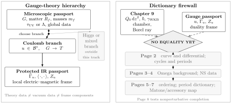
The gauge-theory data firewall. Ultraviolet parameters define the theory, a point $u$ selects a Coulomb vacuum, and a local electric–magnetic frame describes protected infrared data. The dashed arrow from Chapter 9’s WKB passport is deliberately conditional: Pages 2–7 must still construct the Seiberg–Witten curve, differential, cycles, deformation, normalization map, and accessory-parameter relation.

Scope of the chapter

We work in rigid four-dimensional field theory, not supergravity, and focus on the Coulomb branch of Lagrangian $\mathcal N=2$ theories. Higgs and mixed branches, non-Lagrangian theories, defects, and global line-operator refinements enter only where a later ODE dictionary needs them. The symbols $\mathfrak L_{\mathrm{line}}$ and $\vartheta_{\mathrm{disc}}$ in the ultraviolet passport stand for the genuine-line lattice and discrete theta data. Abelian ultraviolet factors and Fayet–Iliopoulos parameters also require extra data and are outside the default setup.

Eight supercharges and two basic multiplets

In four-dimensional Minkowski space, $\mathcal N=2$ means eight real supercharges. Write the independent chiral charges as $Q^A_\alpha$, with spinor index $\alpha=1,2$ and $SU(2)_R$ index $A=1,2$; their Hermitian conjugates are $\bar Q_{\dot\alpha A}$. We choose the central-charge normalization

$$\begin{aligned} \left\{ Q^A_\alpha, \bar Q_{\dot\beta B} \right\} &= 2\sigma^\mu_{\alpha\dot\beta} P_\mu \delta^A{}_B, \\ \left\{ Q^A_\alpha, Q^B_\beta \right\} &= 2\epsilon_{\alpha\beta} \epsilon^{AB}Z. \end{aligned}$$

With this choice, positivity gives the mass inequality

$$M\geq |Z|.$$

Some classic sources absorb a factor $\sqrt2$ into $Z$ and print $M\geq\sqrt2|Z|$. Neither convention is more physical; mixing the algebra from one with the mass formula from the other is an error.

The continuous R-symmetry has local form $SU(2)_R\times U(1)_{\mathsf r}$; globally one often writes

$$U(2)_R \simeq \frac{ SU(2)_R\times U(1)_{\mathsf r} }{\mathbb Z_2}.$$

The subscript $\mathsf r$ labels an R-symmetry and is unrelated to the gauge-group rank $r$. In an asymptotically free theory, the classical $U(1)_{\mathsf r}$ is generally reduced by the anomaly to a discrete subgroup.

The on-shell field content needed here is compact:

Multiplet	Bosons	Fermions	Gauge representation
Vector	Gauge field $A_\mu$ and complex scalar $\phi$	Two Weyl gaugini	Adjoint
Full hypermultiplet	Two complex scalars	Two Weyl fermions	$R\oplus\bar R$

On shell, each massless multiplet has four real bosonic and four real fermionic degrees of freedom. In a pseudoreal representation, a half-hypermultiplet may sometimes be defined; it contributes half as much as a full hypermultiplet to $b_0$ and is subject to global-anomaly constraints. The beta-function formula below is explicitly for full hypermultiplets.

In $\mathcal N=1$ language,

$$\mathcal V_{\mathcal N=2} = V\oplus\Phi, \qquad \mathcal H_R = Q_R\oplus\widetilde Q_{\bar R}.$$

This decomposition is useful because it makes the representations unambiguous. A pure $\mathcal N=2$ Yang–Mills theory contains only the vector multiplet. $\mathcal N=2$ SQCD adds full hypermultiplets in fundamental representations. A complex hypermultiplet mass $m_f$ may be viewed as the scalar expectation value of a nondynamical background vector multiplet for the flavor symmetry.

Supersymmetry constrains quantum corrections strongly, but it does not make the theory free. Charged particles can become light, duality frames can change, BPS states can appear or disappear across walls, and instanton corrections remain. What becomes tractable is a protected low-energy sector.

Vacua are organized by which scalars acquire expectation values. On a Coulomb branch, hypermultiplet vevs vanish while the adjoint scalar varies. On a Higgs branch, hypermultiplet scalars condense and break the gauge group; on a mixed branch, both mechanisms occur. The existence and dimension of the latter branches depend on matter and masses. This chapter follows the Coulomb branch.

The Coulomb branch is a Weyl quotient

Set the hypermultiplet expectation values to zero. The classical potential for the adjoint scalar includes a nonnegative term proportional to

$$\operatorname{tr} \left( [\phi,\phi^\dagger]^\dagger [\phi,\phi^\dagger] \right).$$

A Coulomb vacuum therefore obeys

$$\left[ \phi,\phi^\dagger \right] = 0.$$

A gauge transformation can diagonalize $\phi$ into the complexified Cartan subalgebra $\mathfrak t_{\mathbb C}$, while the Weyl group $W$ still identifies equivalent diagonal values. Thus

$$\mathcal B_{\mathrm{cl}} \simeq \mathfrak t_{\mathbb C}/W, \qquad \dim_{\mathbb C}\mathcal B = r := \operatorname{rank}G.$$

At a regular generic point, every root $\alpha$ satisfies $\alpha(\phi)\neq0$, and the continuous gauge symmetry breaks to a maximal torus:

$$G \longrightarrow T, \qquad \operatorname{Lie}T \simeq \mathfrak u(1)^r.$$

The off-diagonal vector multiplets are massive $W$-multiplets. The massless fields are the $r$ Abelian vector multiplets associated with the Cartan. Classically, root hyperplanes are enhanced-symmetry loci. Quantum effects need not leave those loci in place: the singular set can split or move on the gauge-invariant moduli space.

We use $\Delta\subset\mathcal B$ for the quantum discriminant, where the Abelian low-energy description without extra light fields is singular. It must be removed before choosing one smooth Abelian description:

$$\mathcal B^\circ := \mathcal B\setminus\Delta.$$

Coordinates obtained by diagonalizing $\phi$ are not gauge invariant. Global algebraic coordinates are built from invariant polynomials $P_k$:

$$u_k := \left\langle P_k(\phi) \right\rangle.$$

For $SU(N)$ one commonly uses appropriately normalized traces $u_k\propto\langle\operatorname{tr}\phi^k\rangle$ for $k=2,\ldots,N$. Their precise additive and multiplicative normalizations are part of a later curve convention.

Coulomb is not electric

The phrase Coulomb branch names a family of vacua. It does not select a globally electric duality frame. Near different singularities, the weakly coupled field can be magnetic or dyonic.

The SU(2) quotient in one line of algebra

Fix the trace and scalar conventions

$$\operatorname{tr}_{\mathbf 2} \left( T^aT^b \right) = \frac12\delta^{ab}, \qquad \phi_{\mathrm{cl}} = \begin{pmatrix} a_{\mathrm{cl}}&0\\ 0&-a_{\mathrm{cl}} \end{pmatrix}.$$

Define

$$u := \frac12 \left\langle \operatorname{tr}_{\mathbf2}\phi^2 \right\rangle.$$

Classically,

$$u=a_{\mathrm{cl}}^2.$$

The nontrivial Weyl reflection exchanges the two eigenvalues and sends $a_{\mathrm{cl}}\mapsto-a_{\mathrm{cl}}$. Consequently,

$$\mathcal B_{\mathrm{cl}} = \mathbb C_{a_{\mathrm{cl}}}/\mathbb Z_2 \simeq \mathbb C_u.$$

This elementary quotient already separates a global vacuum coordinate from a local square root. Away from $u=0$, choosing $a_{\mathrm{cl}}$ chooses one of two Weyl-related lifts.

Let $E_\pm$ be the off-diagonal generators. Since

$$\left[ \phi_{\mathrm{cl}},E_\pm \right] = \pm2a_{\mathrm{cl}}E_\pm,$$

the $W^\pm$ multiplets carry electric charge $\pm2$ when a fundamental weight has charge one. In the BPS normalization of this page,

$$M_{W^\pm} = 2|a_{\mathrm{cl}}|.$$

A fundamental hypermultiplet of mass $m$ has two semiclassical color masses

$$|m+a_{\mathrm{cl}}|, \qquad |m-a_{\mathrm{cl}}|.$$

These formulas are classical or weak-coupling statements. Quantum mechanically, $u$ remains gauge invariant, whereas the local infrared coordinate $a(u)$ is only asymptotic to $a_{\mathrm{cl}}$ in a chosen weak-coupling region. The equation $u=a^2$ must not be used globally.

The ultraviolet coupling is not the effective coupling

For each simple gauge factor, define

$$\tau_{\mathrm{UV}} := \frac{\theta}{2\pi} + \frac{4\pi\ii}{g^2}, \qquad q_{\mathrm{UV}} := \ee^{2\pi\ii\tau_{\mathrm{UV}}}.$$

The sign and the factor $2\pi$ in the exponential are now fixed. Elsewhere, the letter $q$ may denote $\ee^{\pi\ii\tau}$, a modular lambda function, or a puncture cross-ratio. A bare symbol $q$ is not a portable convention.

Normalize the representation index by

$$\operatorname{tr}_{R} \left( T^aT^b \right) = T(R)\delta^{ab}, \qquad T(\mathbf N) = \frac12 \quad \text{for }SU(N).$$

For full hypermultiplets in representations $R_f$, the holomorphic one-loop coefficient is

$$b_0 = 2h^\vee(G) - 2\sum_f T(R_f).$$

Hence $SU(N)$ with $N_f$ fundamental full hypers has

$$b_0=2N-N_f.$$

The classification is:

Sign of $b_0$	Ultraviolet behavior	Natural coupling datum
$b_0>0$	Asymptotically free	Dynamically generated scale $\Lambda$
$b_0=0$	Vanishing perturbative beta function	Dimensionless marginal $q_{\mathrm{UV}}$
$b_0<0$	Infrared free as a gauge theory	A UV completion or cutoff is required

For $b_0>0$, one convenient holomorphic definition of the complexified dynamical scale is

$$\Lambda^{b_0} = \mu^{b_0} \ee^{2\pi\ii\tau_{\mathrm{UV}}(\mu)}.$$

Only $\Lambda^{b_0}$ is fixed by this equation. Choosing $\Lambda$ itself also chooses a $b_0$-th-root branch, and its multiplicative normalization is scheme-dependent. For pure $SU(2)$, $b_0=4$ and

$$\Lambda^4 = \mu^4 \ee^{2\pi\ii\tau_{\mathrm{UV}}(\mu)}.$$

With $N_f$ fundamental hypers, $b_0=4-N_f$: the cases $N_f=0,1,2,3$ are asymptotically free, and $N_f=4$ is conformal before masses are introduced.

Extended supersymmetry makes the Wilsonian perturbative running one-loop exact. It does not remove nonperturbative corrections to the low-energy theory. Nor should $\tau_{\mathrm{UV}}$ be confused with the vacuum-dependent matrix of effective Abelian couplings $\tau_{ij}^{\mathrm{eff}}(u)$.

Holomorphy controls the local two-derivative theory

At $u\in\mathcal B^\circ$, integrate out fields that are heavy compared with the probe scale. The remaining two-derivative theory contains $r$ Abelian vector multiplets. In a local electric frame, its scalar coordinates are $a^i$. $\mathcal N=2$ supersymmetry packages the effective couplings and scalar metric into holomorphic data, locally described by a prepotential $\mathcal F$ in that chosen frame.

The word local is essential. Electric–magnetic duality changes the coordinates and the prepotential chart. A single $\mathcal F(a)$ need not be a global holomorphic function on all of $\mathcal B^\circ$. Page 2 defines the derivatives of $\mathcal F$, constructs the dual coordinates and their symplectic transitions, and derives the Seiberg–Witten periods and scalar metric that make this geometry explicit.

This is also a Wilsonian two-derivative statement. Higher-derivative operators are present, and the one-particle-irreducible action can have additional infrared subtleties when massless particles propagate.

Charges form a local system, not one global list

Let $\widehat\Gamma_u$ denote the lattice of gauge and flavor charges at a regular vacuum. Here “charge” means a dynamical particle or flavor charge label; the hat reminds us that flavor charges are included. The antisymmetric Dirac–Schwinger–Zwanziger pairing can have a radical: pure flavor charges pair trivially with every charge. After quotienting that radical, the dynamical electromagnetic lattice has rank $2r$ and a nondegenerate integral skew pairing. More precisely, assuming there are no additional decoupled radical directions, set

$$\Gamma_{\mathrm f,u} = \operatorname{rad} \langle\,\cdot,\cdot\,\rangle_u, \qquad \Gamma_{\mathrm{em},u} = \widehat\Gamma_u/\Gamma_{\mathrm f,u}.$$

The electromagnetic pairing need not be unimodular. Its elementary divisors are physical integral data, not artifacts of a complex change of frame.

Equivalently, there is an extension

$$0 \longrightarrow \Gamma_{\mathrm f,u} \longrightarrow \widehat\Gamma_u \longrightarrow \Gamma_{\mathrm{em},u} \longrightarrow 0.$$

Fiberwise, these sequences assemble into local systems over $\mathcal B^\circ$. Choose a local splitting and an integral basis of $\Gamma_{\mathrm{em}}$ adapted to its elementary divisors. Separately, it is often useful to place the dynamical lattice inside an integral period or probe lattice on which the central charge extends:

$$\begin{gathered} \Gamma_{\mathrm{em},u} \hookrightarrow \Gamma_{\mathrm{per},u}, \\ \widehat\Gamma_u \hookrightarrow \widehat\Gamma_{\mathrm{per},u} := \Gamma_{\mathrm{per},u} \oplus \Gamma_{\mathrm f,u}, \end{gathered}$$

where the second line uses the chosen local flavor splitting. The dynamical electromagnetic and period lattices can coincide, but they need not. A principal period lattice admits unit-paired basis classes $E_i,M^i$ with $\langle E_i,M^j\rangle=\delta_i{}^j$; the dynamical charges may obey congruence restrictions in that basis. “Probe” here means a charge used to normalize the low-energy Abelian fields, not automatically a genuine Wilson–’t Hooft line operator. Page 2 will show explicitly that, in the unit-electric-probe normalization of pure $SU(2)$, $\Gamma_{\mathrm{em}}=\langle2E,M\rangle$ sits with index two inside $\Gamma_{\mathrm{per}}=\langle E,M\rangle$.

Relative to a principal period frame, write a dynamical charge as

$$\gamma = \left( \boldsymbol n_e, \boldsymbol n_m; \boldsymbol s \right).$$

Here $(\boldsymbol n_e,\boldsymbol n_m)$ are restricted to the dynamical sublattice when $\Gamma_{\mathrm{em}}$ is proper. The flavor splitting is generally noncanonical: a lift of an electromagnetic charge may shift by a flavor charge. Such a change is compensated by mass-dependent shifts in the displayed frame coordinates and leaves $Z_\gamma$ invariant.

Our pairing convention in this unit period frame is

$$\left\langle \gamma,\gamma' \right\rangle = \boldsymbol n_e\mathbin{\cdot}\boldsymbol n_m' - \boldsymbol n_m\mathbin{\cdot}\boldsymbol n_e'.$$

The central charge is the additive homomorphism

$$\begin{aligned} Z_\gamma(u) ={}& \boldsymbol n_e\mathbin{\cdot}\boldsymbol a(u) + \boldsymbol n_m\mathbin{\cdot}\boldsymbol a_D(u) \\ &+ \boldsymbol s\mathbin{\cdot}\boldsymbol m. \end{aligned}$$

At this stage, $a^i$ and $a_{D,i}$ are defined abstractly as the values of the extended central-charge section on the period basis $E_i,M^i$. They restrict to the physical central charges of every dynamical particle label, but a unit period-basis class need not itself be a dynamical particle charge. Page 2 will realize these coordinates as periods and relate them to the prepotential.

As $u$ moves around a noncontractible loop in $\mathcal B^\circ$, the charge basis can return by an integral pairing-preserving automorphism of $\widehat\Gamma$. A compatible period lattice has its own integral pairing-preserving monodromy, preserving the embedded dynamical sublattice. Thus $\widehat\Gamma\to\mathcal B^\circ$ is a local system, while $a$, $a_D$, and the components of $\gamma$ are frame-dependent. The number $Z_\gamma$ is invariant when the central-charge vector and charge components are transformed contragrediently.

Because a full pairing-preserving monodromy may also mix a chosen electromagnetic lift with flavor charge, period components can acquire mass-dependent affine shifts. The induced action on $\Gamma_{\mathrm{em}}$ continues to preserve its integral skew form, whether or not that form is principal.

Pairing orientation

Some sources reverse the sign of the Dirac pairing or order the central-charge vector as $(a,a_D)^T$ instead of $(a_D,a)^T$. Either convention is consistent. A comparison must transform the charge vector, central-charge vector, and monodromy matrices together.

BPS saturation does not populate the spectrum

The central extension of the supersymmetry algebra implies

$$M_\gamma\geq |Z_\gamma|.$$

A one-particle state that saturates the inequality is BPS. Its representation is shorter than a generic massive $\mathcal N=2$ multiplet. Shortening makes the equality

$$M_\gamma^{\mathrm{BPS}} = |Z_\gamma|.$$

exact, although $Z_\gamma(u)$ is quantum-corrected and varies over moduli space. The formula is conditional on the state existing. The charge lattice lists allowed charge labels; it is not a catalogue of particles. Stability can change on a wall of marginal stability, where possible constituents have aligned phases:

$$\arg Z_{\gamma_1} = \arg Z_{\gamma_2}.$$

Across such a wall, a BPS index may jump even though the holomorphic central charges vary smoothly. Likewise, $Z_\gamma(u_*)=0$ signals a massless particle only if a BPS state of charge $\gamma$ is actually present in the relevant chamber. The discriminant records singular low-energy physics, not every formal zero of every linear function on the charge lattice.

This distinction mirrors Chapter 9. An allowed WKB cycle does not by itself impose a boundary condition, and an allowed gauge charge does not by itself guarantee a stable particle.

The WKB–gauge dictionary is still conditional

The structural parallels can now be stated without turning them into identities:

Exact-WKB object from Chapters 8–9	Gauge-theory object on this page	Present status
Anti-invariant cycle lattice and intersection form	Electromagnetic lattice and Dirac pairing	Analogy; equality requires Page 2’s curve and cycle map
Classical period $Z_\gamma^{\mathrm{WKB}}=\oint_\gamma\lambda_0$	Abstract central charge $Z_\gamma(u)$	Not yet identified
Puncture loops and residues	Flavor charges and masses	Common relation, with model-dependent factors and shifts
Energy or accessory parameter	Coulomb modulus $u_k$	Common in examples, never universal
Stokes or Borel chamber	BPS stability chamber	Related in specified geometric constructions, not generically synonymous
WKB parameter $\hbar$	No undeformed $4d$ quantity	Candidate $\epsilon_1$ appears only after Pages 3–4
Exact quantization determinant	Bethe-vacuum or gauge-theory condition	Requires Pages 5–8 and may need nonperturbative completion

The shared symbol $Z_\gamma$ is intentional: both sides attach a complex number linearly to a charge or cycle. It does not license the equality

$$Z_\gamma^{\mathrm{WKB}} \stackrel{?}{=} Z_\gamma^{\mathrm{SW}}$$

until the spectral curve, Seiberg–Witten differential, cycle orientation, parameter map, and normalization have all been fixed.

No undeformed hbar

Undeformed Seiberg–Witten theory has no independent deformation parameter identified with the ODE’s WKB $\hbar$. Writing $\hbar=\epsilon_1$ before introducing the Omega background and taking the Nekrasov–Shatashvili limit silently skips Pages 3–4.

Common pitfalls

Using $u$ and $a$ interchangeably. The $u_k$ are gauge-invariant coordinates on the Coulomb branch. The $a^i$ are local infrared coordinates in an electric frame; even for $SU(2)$, $u=a_{\mathrm{cl}}^2$ is only the classical relation.

Treating $\tau_{\mathrm{UV}}$ as $\tau_{\mathrm{eff}}(u)$. The first defines the microscopic coupling or conformal modulus. The second is a vacuum-dependent Abelian coupling derived from the low-energy prepotential.

Inferring a particle from an integral charge. Charge quantization specifies allowed labels. It does not prove that a stable BPS state occupies every lattice point in every chamber.

Ignoring the flavor radical. Flavor charges contribute $\boldsymbol s\cdot\boldsymbol m$ to $Z_\gamma$ but pair trivially under the gauge Dirac pairing. Calling the full charge lattice symplectic without quotienting its radical is imprecise.

Comparing formulas before comparing conventions. Factors of $\sqrt2$, the order of $(a_D,a)$, the sign of the Dirac pairing, the definition of $q$, and the scale normalization all vary in standard sources.

Equating structural analogy with correspondence. Similar skew lattices and central charges motivate the Seiberg–Witten/WKB map. They do not determine the curve, differential, operator ordering, mass shifts, or spectral completion.

Exercises

1. Count the supercharges

Why do the operators $Q^A_\alpha$ describe eight real supercharges rather than four or sixteen? What role do $\bar Q_{\dot\alpha A}$ play?

Solution

The indices $A=1,2$ and $\alpha=1,2$ give four complex components. Four complex components are eight real components. The barred charges are their Hermitian conjugates in Minkowski signature, not eight new independent real generators. Thus the total is eight real supercharges.

2. Recover the SU(2) Weyl quotient

Show that every polynomial invariant of $\phi=\operatorname{diag}(a_{\mathrm{cl}},-a_{\mathrm{cl}})$ is a polynomial in $a_{\mathrm{cl}}^2$. Why is $a_{\mathrm{cl}}$ double-valued over the $u$-plane?

Solution

The Weyl group is $\mathbb Z_2$ and acts by $a\mapsto-a$. A polynomial

$$f(a_{\mathrm{cl}}) = \sum_{k\geq0}c_k a_{\mathrm{cl}}^k$$

is invariant precisely when $f(-a_{\mathrm{cl}})=f(a_{\mathrm{cl}})$, so all odd coefficients vanish. Therefore $f(a_{\mathrm{cl}})=g(a_{\mathrm{cl}}^2)$ for a polynomial $g$. With $u=a_{\mathrm{cl}}^2$, a regular value $u\neq0$ has the two lifts $a_{\mathrm{cl}}=\pm\sqrt u$, exchanged by the Weyl reflection. The branch point at $u=0$ is the classical enhanced-symmetry point.

3. Derive the charged SU(2) masses

Using $\phi_{\mathrm{cl}}=\operatorname{diag}(a_{\mathrm{cl}}, -a_{\mathrm{cl}})$, derive the $W$-multiplet charges and the two semiclassical masses of a fundamental hypermultiplet of mass $m$.

Solution

For the matrix units $E_{12}$ and $E_{21}$,

$$\begin{aligned} [\phi_{\mathrm{cl}},E_{12}] &= 2a_{\mathrm{cl}}E_{12}, \\ [\phi_{\mathrm{cl}},E_{21}] &= -2a_{\mathrm{cl}}E_{21}. \end{aligned}$$

If a fundamental weight has electric charge one, the two off-diagonal fields have charges $\pm2$. Their central charges are $\pm2a_{\mathrm{cl}}$, hence their BPS masses are $2|a_{\mathrm{cl}}|$.

On the fundamental representation, $\phi_{\mathrm{cl}}$ has eigenvalues $\pm a_{\mathrm{cl}}$. Adding the flavor mass shifts the complex masses to $m\pm a_{\mathrm{cl}}$, so the physical masses are $|m+a_{\mathrm{cl}}|$ and $|m-a_{\mathrm{cl}}|$.

4. Generalize the classical count to SU(N)

For

$$\phi_{\mathrm{cl}} = \operatorname{diag}(v_1,\ldots,v_N), \qquad \sum_{i=1}^N v_i=0,$$

count the Coulomb-branch dimension, identify the $W$-boson mass differences, and give $b_0$ for $N_f$ fundamental full hypers.

Solution

The traceless condition leaves $N-1$ independent eigenvalues, and permutations by the Weyl group $S_N$ do not change the complex dimension. Thus

$$\dim_{\mathbb C}\mathcal B=N-1.$$

The root associated with the matrix unit $E_{ij}$ evaluates to $v_i-v_j$, so the off-diagonal multiplet has semiclassical mass $|v_i-v_j|$ in the corresponding normalization. A coincidence $v_i=v_j$ is a classical enhanced-symmetry locus.

Since $h^\vee(SU(N))=N$ and each fundamental has index $1/2$,

$$b_0 = 2N-N_f.$$

The theory is asymptotically free for $N_f<2N$ and has vanishing perturbative beta function for $N_f=2N$.

5. Classify SU(2) matter theories

Compute $b_0$ for $SU(2)$ with $N_f=0,\ldots,5$ fundamental full hypermultiplets. Classify the ultraviolet behavior and check the mass dimension of $\Lambda$ when $b_0>0$.

Solution

For $SU(2)$, $h^\vee=2$ and each fundamental has $T(\mathbf2)=1/2$. Therefore

$$b_0 = 4-N_f.$$

$N_f$	$b_0$	Behavior
$0$	$4$	Asymptotically free
$1$	$3$	Asymptotically free
$2$	$2$	Asymptotically free
$3$	$1$	Asymptotically free
$4$	$0$	Exactly conformal when all masses vanish; otherwise a mass deformation with zero gauge beta function
$5$	$-1$	Infrared free as a gauge theory

In

$$\Lambda^{b_0} = \mu^{b_0}q_{\mathrm{UV}}(\mu),$$

$q_{\mathrm{UV}}$ is dimensionless. Hence $[\Lambda^{b_0}]=[\mu^{b_0}]$, so $[\Lambda]=1$ for $b_0>0$.

6. Sort the data before computing

Classify

$$m_f,\quad \Lambda,\quad u_k,\quad a^i,\quad a_{D,i},\quad \gamma,\quad \hbar$$

as ultraviolet parameter, vacuum coordinate, derived local infrared quantity, charge label, or not-yet-present deformation parameter.

Solution

Symbol	Role
$m_f$	Ultraviolet flavor-mass parameter
$\Lambda$	Ultraviolet RG-invariant scale of an asymptotically free theory
$u_k$	Gauge-invariant Coulomb-vacuum coordinate
$a^i$, $a_{D,i}$	Derived local infrared central-charge coordinates
$\gamma$	Integral gauge–flavor charge label
$\hbar$	Not present in the undeformed theory; later identified conditionally with an Omega-background parameter

The entries are related, but they are not interchangeable. In particular, fixing the theory data does not fix $u$, and fixing $u$ does not choose one global electric frame.

7. Pair elementary electric and magnetic period classes

At rank one, choose a principal period/probe frame and take

$$\gamma_e=(1,0;0), \qquad \gamma_m=(0,1;0),$$

where the entries are $(n_e,n_m;s)$. Compute their pairing and central charges. Must both classes be dynamical particle charges? Which local coordinate must vanish for a magnetic BPS state to become massless?

Solution

The declared convention gives

$$\langle\gamma_e,\gamma_m\rangle = 1.$$

Their central charges are

$$Z_{\gamma_e}=a, \qquad Z_{\gamma_m}=a_D.$$

These are unit period-basis classes; a theory’s dynamical lattice may contain only a sublattice. In the pure-$SU(2)$ convention of Page 2, for example, $\gamma_e$ is a unit probe while $2\gamma_e$ and $\gamma_m$ are dynamical charge generators. A BPS state of pure magnetic charge has mass $|a_D|$, so it becomes massless where $a_D=0$, provided that state exists in the chamber. The condition $a=0$ instead concerns the chosen electric period class.

8. Verify frame covariance

Order the rank-one infrared central-charge vector as

$$\Pi = \begin{pmatrix} a_D\\ a \end{pmatrix} .$$

For vanishing flavor charge, the row $q=(n_m,n_e)$ is the reordered packaging of the earlier label $\gamma=(n_e,n_m;0)$, so $Z=q\Pi$. Under

$$S = \begin{pmatrix} 0&-1\\ 1&0 \end{pmatrix}, \qquad \Pi'=S\Pi, \qquad q'=qS^{-1},$$

show that the central charge is unchanged.

Solution

The transformed data are

$$\Pi' = \begin{pmatrix} -a\\ a_D \end{pmatrix}, \qquad q' = (-n_e,n_m).$$

Therefore

$$q'\Pi' = (-n_e)(-a)+n_ma_D = n_ea+n_ma_D = q\Pi.$$

The components changed, but the physical central charge did not. This is why a central-charge vector cannot be transformed without simultaneously transforming charge labels and monodromy conventions.

9. Locate a marginal-stability wall

Suppose a state of charge $\gamma=\gamma_1+\gamma_2$ can decay into two BPS constituents. Derive the condition under which the BPS mass bound allows threshold decay.

Solution

Linearity gives

$$Z_\gamma = Z_{\gamma_1}+Z_{\gamma_2}.$$

The triangle inequality implies

$$|Z_\gamma| \leq |Z_{\gamma_1}|+|Z_{\gamma_2}|.$$

Equality holds exactly when the two nonzero central charges have the same phase:

$$\arg Z_{\gamma_1} = \arg Z_{\gamma_2}.$$

This is the marginal-stability condition. It permits a threshold decay but does not determine on which side the bound state exists; that requires dynamical BPS-index data.

10. Audit a premature ODE dictionary

A proposed calculation declares

$$E=u=a^2, \qquad \hbar=\epsilon_1, \qquad \oint_\gamma p\,\dd x=Z_\gamma,$$

solely because both descriptions contain periods. List the missing data and identify which later pages supply them.

Solution

The proposal has silently omitted:

1. a specific Seiberg–Witten curve and differential—Page 2;
2. an oriented identification of WKB cycles with electric–magnetic cycles—Page 2 and Page 6;
3. the normalization and possible mass-dependent shift relating $E$ to the gauge-invariant modulus $u$—Pages 5–7;
4. the distinction between global $u$ and local $a$—Pages 1–2;
5. the Omega-background convention for $(\epsilon_1,\epsilon_2)$ and the NS limit—Pages 3–4;
6. quantum-curve ordering, polarization, and the quantum mirror map—Pages 5–6; and
7. the difference between all-orders NS data and a nonperturbative spectrum—Page 8.

Until these items are fixed, the three displayed equalities are mnemonics, not mathematical statements.

Geometry comes next

We now have an abstract infrared package:

$$\left( \widehat\Gamma_u, \langle\,\cdot,\cdot\,\rangle, Z_u \right), \qquad u\in\mathcal B^\circ.$$

Together with a declared local realization in $\widehat\Gamma_{\mathrm{per},u}$, Page 2 asks how a family of algebraic curves and a meromorphic Seiberg–Witten differential realize this package as cycle periods. That step will introduce $A/B$ cycles, special coordinates, monodromy, and the rigid special Kähler structure. Only after the dynamical and period lattices and their normalizations are fixed can the WKB cycle lattice be compared with the electromagnetic one.

References

• Seiberg, N., and Witten, E., “Electric–Magnetic Duality, Monopole Condensation, and Confinement in $\mathcal N=2$ Supersymmetric Yang–Mills Theory”, Nuclear Physics B 426 (1994), 19–52; erratum 430 (1994), 485–486. Sections 2.1–2.3 develop the multiplets, flat directions, and Abelian effective action; §4 treats central charges and BPS masses in the paper’s original normalization.
• Seiberg, N., and Witten, E., “Monopoles, Duality and Chiral Symmetry Breaking in $\mathcal N=2$ Supersymmetric QCD”, Nuclear Physics B 431 (1994), 484–550. The convention note; §§2–3 cover hypermultiplets and classical $SU(2)$ SQCD, §4.1 treats running, and §5 develops the BPS states.
• Witten, E., and Olive, D. I., “Supersymmetry Algebras That Include Topological Charges”, Physics Letters B 78 (1978), 97–101. Foundational source for central extensions and the protected soliton mass bound.
• Tachikawa, Y., N=2 Supersymmetric Dynamics for Pedestrians, Lecture Notes in Physics 890 (2015). Sections 2.1–2.4 give the field-theory and BPS background; §3.1 fixes running and $\Lambda$; §4.1 uses the $u\sim a^2$, $M_W=2|a|$ convention adopted here; see §§2.2 and 4.1.
• D’Hoker, E., and Phong, D. H., “Lectures on Supersymmetric Yang–Mills Theory and Integrable Systems”, in Theoretical Physics at the End of the Twentieth Century (2002), 1–125. Lectures I–II provide a systematic treatment of multiplets, holomorphy, duality, and Seiberg–Witten theory.
• Bilal, A., “Duality in $\mathcal N=2$ SUSY $SU(2)$ Yang–Mills Theory: A Pedagogical Introduction to the Work of Seiberg and Witten”, in Quantum Fields and Quantum Space Time (1997), 21–43. Sections 2–4 give a detailed pedagogical derivation; §6.1 is especially useful for readers approaching the subject from differential equations.
• Gaiotto, D., Moore, G. W., and Neitzke, A., “Wall-Crossing, Hitchin Systems, and the WKB Approximation”, Advances in Mathematics 234 (2013), 239–403. Section 2.1 formulates the charge local system, flavor radical, pairing, and central charge; the later WKB realization applies to the class of theories constructed there.
• Aharony, O., Seiberg, N., and Tachikawa, Y., “Reading Between the Lines of Four-Dimensional Gauge Theories”, Journal of High Energy Physics 08 (2013), 115. Sections 1.1–1.2 explain why the global gauge-group form and allowed line operators refine the electromagnetic charge lattice.