Polynomial and Exponential Potentials

The homogeneous oscillator of Pages 4–6 is unusually economical. A Symanzik step rotates the energy but leaves the potential passport fixed, so one determinant reappears at shifted arguments. Lower polynomial couplings usually destroy that one-function picture without destroying the underlying ODE identities: the rotation now visits a finite list of different operators, and their determinants satisfy a coupled system.

Exponential potentials reveal the same geometry in another coordinate. After $x=\ee^t$, a complex rotation of $x$ is an imaginary translation of $t$. Whether repeated translations return the coefficient passport is an arithmetic question about the exponents. Even when they do, a Baxter or transfer-matrix interpretation still requires a named integrable model, state, spectral scale, and analytic passport.

This page develops that hierarchy. It begins with exact ODE covariance, isolates a polynomial deformation for which a two-component TQ system is known, and then carries the construction to exponential coordinates. It does not derive a nonlinear integral equation; the zero locations, analyticity strips, and contour deformations needed for that step begin in Chapter 13.

The closure test

Apply one covariance step to the nonspectral passport: coefficients, canonical lines, contour, sheet, and normalization. Record separately how the spectral coordinate, such as $E$ or $\theta$, shifts.

• If the nonspectral passport returns after one step, a scalar relation may close on one determinant evaluated at shifted spectral arguments.
• If it returns after $L>1$ steps, the natural object is an $L$-component orbit of determinant families.
• If it never returns, covariance still gives exact identities, but not a finite functional system.

Closure is an ODE statement. Calling the resulting functions $T$, $Q$, or $Y$ is a further, model-dependent identification. Return of one numerical spectral point is a different question and does not count the components.

Status ledger

Statement	Status
Symanzik action on a polynomial coefficient passport	Exact substitution
Adjacent-orbit bilinear for raw endpoint functions	Exact Wronskian identity in the Page 3 gauge
A finite orbit for an integer-degree polynomial	Exact; generically its length is degree plus two, with symmetry reductions possible
Scalar closure for a homogeneous potential	Exact ODE closure; its BLZ interpretation is the model-specific result of Pages 4–5
The two-component relation for $x^{2M}+\alpha x^{M-1}+l(l+1)/x^2$	Exact ODE identity; Suzuki and Dorey–Dunning–Tateo develop model-specific functional interpretations in stated conventions
Coupled root equations	Exact after the relevant determinant is entire, factorized, and the divided denominator is nonzero
Logarithmic Liouville transformation and boundary-line map	Exact coordinate and gauge transformation on a chosen logarithmic sheet
Finite fixed-coefficient closure for a sum of exponentials with commensurate exponents	Exact coefficient-orbit statement; it does not prove spectral analyticity or an IM dictionary
Generalized Mathieu QQ and dual TQ relations	Exact Wronskian identities in the explicitly stated source normalization
Massive sine–/sinh–Gordon Q-functions from modified sinh–Gordon	Conditional on the specified nonlinear background, auxiliary system, global hypotheses, and branch of the correspondence

A generic polynomial closes on an operator orbit

Retain the even-degree family and normalization of Page 3,

$$\begin{aligned} \left[-\frac{\dd^2}{\dd x^2}+P(x;g)\right]y &=Ey, \\ P(x;g) &=x^{2M}+\sum_{a=0}^{2M-1}g_ax^a, \qquad M\in\mathbb N, \quad M>1. \end{aligned}$$

Put

$$\omega=\ee^{\pi\ii/(M+1)}, \qquad \mathfrak p=(E,\{g_a\}),$$

and let the one-step parameter map be

$$\mathcal R\mathfrak p = \left( \omega^2E, \{\omega^{a+2}g_a\}_{a=0}^{2M-1} \right).$$

The constant coefficient and $E$ have the same weight; only $g_0-E$ enters the differential equation. Let $b(\mathfrak p)$ be the coefficient of $x^{-1}$ in the large-$x$ expansion of $\sqrt{P(x;g)-E}$. In the adjacent-Wronskian gauge,

$$y_1(x;\mathfrak p) = \omega^{1/2+b(\mathfrak p)} y_0\!\left(\omega^{-1}x;\mathcal R\mathfrak p\right),$$

and

$$\Wr[y_0,y_1]=2\ii.$$

At an ordinary origin define the raw endpoint functions

$$A(\mathfrak p)=y_0(0;\mathfrak p), \qquad B(\mathfrak p)=y_0'(0;\mathfrak p).$$

Evaluation of the adjacent Wronskian at zero gives the exact bilinear

$$\begin{aligned} &\omega^{b-1/2} A(\mathfrak p)B(\mathcal R\mathfrak p) \\ &\quad- \omega^{b+1/2} B(\mathfrak p)A(\mathcal R\mathfrak p) =2\ii, \end{aligned}$$

where $b=b(\mathfrak p)$. This is the polynomial analogue of a quantum Wronskian before any integrable-model names are attached. It couples the raw Dirichlet boundary function $A$ of one operator to the raw Neumann boundary function $B$ of its rotated partner. In Voros’s convention one may write

$$\Delta^-_{\mathrm{raw}}=A, \qquad \Delta^+_{\mathrm{raw}}=-B.$$

By contrast, the Page 1 determinants are

$$\begin{aligned} D_{\mathrm D}(E;g) &=\frac{A(E;g)}{A(0;g)}, \\ D_{\mathrm N}(E;g) &=\frac{B(E;g)}{B(0;g)}, \end{aligned}$$

provided the two denominators are nonzero. Thus zero-energy factors cannot be dropped when the couplings rotate.

Because every coefficient weight is integral,

$$\mathcal R^{2M+2}\mathfrak p=\mathfrak p.$$

More precisely, set $L_g=1$ when all lower couplings vanish; otherwise the coefficient orbit has length

$$L_g =\operatorname{lcm}_{g_a\ne0} \frac{2M+2}{\gcd(2M+2,a+2)}.$$

If one asks when the full numerical point $(E,g)$ returns, the energy weight $2$ must also be included in the least common multiple. The oriented sector orbit still has $2M+2$ steps even when the coefficient orbit is shorter. These are three distinct returns: coefficients, a numerical parameter point, and a canonically normalized sectorial representative.

Thus there are at most $2M+2$ adjacent bilinears. The effective determinant system can be shorter when the coefficient pattern has extra symmetry. For a general monic polynomial of degree $N$, the analogous construction has $N+2$ partners; the even-degree notation above is kept to preserve the Page 3 normalization and sector labels.

The important point is negative as well as positive. A finite list of exact determinant identities does not imply that each determinant is an eigenvalue of one Baxter operator. Generically the list belongs to different complex-scaled Schrödinger operators.

The even quartic needs three coupling passports

Consider

$$P(x;g)=x^4+gx^2, \qquad \omega=\ee^{\pi\ii/3}, \qquad j=\omega^2=\ee^{2\pi\ii/3}.$$

Here $b=0$. Both $E$ and $g$ have a three-step coefficient orbit; equivalently, parity identifies opposite members of the six-step canonical-sector orbit in the endpoint chain. The three passports are

$$\begin{array}{c|c|c} r&E^{[r]}&g^{[r]} \\ \hline 0&E&g \\ 1&jE&j^2g \\ 2&j^2E&jg. \end{array}$$

Writing $A_r=A(\mathcal R^r\mathfrak p)$ and $B_r=B(\mathcal R^r\mathfrak p)$, the three cyclic links are

$$\omega^{-1/2}A_rB_{r+1} -\omega^{1/2}B_rA_{r+1} =2\ii, \qquad r\pmod 3.$$

For $g\ne0$, the three spectra belong to the couplings $g,j^2g,jg$. At $g=0$ those coupling passports coincide, and the system collapses to the homogeneous scalar relation used earlier in the chapter. This limiting collapse, rather than a change of notation, explains why the pure quartic is exceptional.

One relevant deformation produces a two-component TQ system

A particularly useful lower monomial has precisely the weight needed to change sign under one Symanzik step:

$$\begin{aligned} H_\sigma(M,\alpha,l) ={}&-\frac{\dd^2}{\dd x^2} +x^{2M} +\sigma\alpha x^{M-1} +\frac{l(l+1)}{x^2}, \\ &\sigma\in\{+1,-1\}. \end{aligned}$$

Indeed,

$$\omega^{M+1}=-1,$$

so a rotation interchanges $H_+$ and $H_-$ while sending $E\mapsto\omega^2E$. Assume first $\Re l>-1/2$ and a nonresonant Frobenius pair. Let $y_0(x,E,\sigma\alpha,l)$ be the canonical solution at infinity, and normalize $\psi_+\sim x^{l+1}$ to leading coefficient one. For real $l>-1/2$, this is the regular/Friedrichs radial line. Other values can be reached by analytic continuation; resonant cases require a separate logarithmic prescription. Define

$$\begin{aligned} D_\sigma(E) &:=\Wr[y_0(E,\sigma\alpha,l),\psi_+], \\ T_\sigma(E) &:=\frac{1}{2\ii} \Wr[y_{-1}(E,\sigma\alpha,l), y_1(E,\sigma\alpha,l)]. \end{aligned}$$

The subscript $\sigma$ records the sign of the polynomial deformation. It is not the $Q_\pm$ label for the two Frobenius branches on Pages 4–6.

Put

$$\kappa_\sigma =\frac{2l+1+\sigma\alpha}{2}.$$

Taking the Wronskian of $T_\sigma y_0=y_{-1}+y_1$ with $\psi_+$ and transporting the normalized power $x^{l+1}$ through the two rotations gives

$$\boxed{ \begin{aligned} T_\sigma(E)D_\sigma(E) ={}& \omega^{-\kappa_\sigma} D_{-\sigma}(\omega^{-2}E) \\ &+ \omega^{\kappa_\sigma} D_{-\sigma}(\omega^2E). \end{aligned} }$$

This is a genuine two-component TQ-type system: one equation at $+\alpha$, one at $-\alpha$. The coefficient phases combine the Frobenius power $l+1$, the derivative Jacobian, and the logarithmic WKB power $\sigma\alpha/2$. Omitting any one of those three contributions changes $\kappa_\sigma$.

The displayed $D_\sigma$ are raw connection Wronskians. Assume

$$D_+(0)D_-(0)\ne0.$$

If each branch is independently normalized by

$$\widehat D_\sigma(E) =\frac{D_\sigma(E)}{D_\sigma(0)},$$

then the right-hand side of the boxed equation is multiplied by

$$r_\sigma =\frac{D_{-\sigma}(0)}{D_\sigma(0)}.$$

The homogeneous phases cannot be retained while this unequal zero-energy factor is silently discarded.

Let $E_{k,\sigma}$ be a zero of $D_\sigma$. If neither shifted value of $D_{-\sigma}$ vanishes, evaluation at the root gives

$$\frac{ D_{-\sigma}(\omega^2E_{k,\sigma}) }{ D_{-\sigma}(\omega^{-2}E_{k,\sigma}) } =- \omega^{-(2l+1+\sigma\alpha)}.$$

For $M>1$, a genus-zero product then yields the coupled Bethe-root form

$$\prod_{n=0}^{\infty} \frac{ E_{n,-\sigma}-\omega^2E_{k,\sigma} }{ E_{n,-\sigma}-\omega^{-2}E_{k,\sigma} } =- \omega^{-(2l+1+\sigma\alpha)}.$$

The zeros of one connection function are constrained by the entire zero set of its partner. On a declared self-adjoint real radial domain, those zeros are spectra. At $\alpha=0$, $D_+=D_-$ and the two equations collapse to the single homogeneous system. For nonzero $\alpha$, replacing both determinants by the same symbol loses physical data.

For $M=3$, $l=0$, and real $\alpha>0$, the two full-line potentials are

$$V_+(x)=x^6+\alpha x^2, \qquad V_-(x)=x^6-\alpha x^2.$$

The first is a single well. The second has a local maximum at zero and minima at $x=\pm(\alpha/3)^{1/4}$. The functional relation couples their half-line determinants; it does not assert that the two spectra are equal.

The ODE identities above are exact. For this deformation Suzuki identified a hidden $U_q(\widehat{\mathfrak{gl}}(2|1))$ fusion structure and coupled nonlinear integral equations, while Dorey–Dunning–Tateo extended the functional system to include $l$. On this page “TQ-type” describes the algebraic form. NLIE characterization, uniqueness, and completeness require the analytic and root-location hypotheses stated in those works; none follows for arbitrary lower couplings merely because their Symanzik orbit is finite.

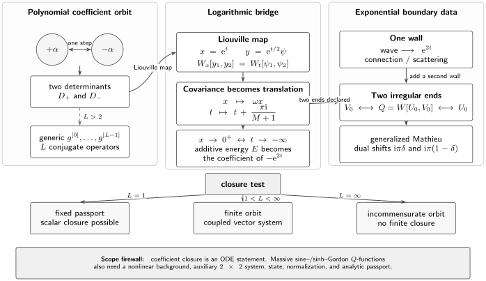
Covariance has three algebraic outcomes. A fixed passport can support a scalar shifted relation; a finite nontrivial orbit produces a vector of coupled determinants; an infinite orbit does not close finitely. The massive sine–/sinh–Gordon correspondence is a separate branch: its $Q$ function is a connection coefficient of a linear system over a specified modified sinh–Gordon background, not a relabeled determinant of every scalar exponential potential.

A logarithm turns rotations into imaginary translations

The polynomial and exponential descriptions are joined by an exact Liouville transformation. Set

$$x=\ee^t, \qquad y(x)=\ee^{t/2}\psi(t).$$

For any two transformed solutions the gauge factor cancels the derivative Jacobian exactly:

$$\Wr_x[y_1,y_2] =\Wr_t[\psi_1,\psi_2].$$

Then

$$\begin{aligned} &\left[ -\frac{\dd^2}{\dd x^2} +x^{2M} +\alpha x^{M-1} +\frac{l(l+1)}{x^2} \right]y=Ey \end{aligned}$$

is equivalent, on the chosen logarithmic sheet, to

$$\begin{aligned} \biggl[ -\frac{\dd^2}{\dd t^2} &+\ee^{2(M+1)t} +\alpha\ee^{(M+1)t} \\ &-E\ee^{2t} +\left(l+\frac12\right)^2 \biggr]\psi=0. \end{aligned}$$

Two conceptual roles have moved:

• the half-line $x\in(0,\infty)$ is the full real $t$-axis;
• $E$ is now the coefficient of $-\ee^{2t}$, not an additive eigenvalue on the right-hand side.

The transformation is Wronskian-preserving but not unitary in the flat $t$ measure:

$$\int_0^\infty |y(x)|^2\,\dd x =\int_{-\infty}^{\infty} \ee^{2t}|\psi(t)|^2\,\dd t.$$

The radial origin line becomes an asymptotic line at $t\to-\infty$:

$$\begin{aligned} y\sim x^{l+1} &\quad\Longleftrightarrow\quad \psi\sim\ee^{(l+1/2)t}, \\ y\sim x^{-l} &\quad\Longleftrightarrow\quad \psi\sim\ee^{-(l+1/2)t}. \end{aligned}$$

The canonical recessive line at $x\to+\infty$ becomes the recessive line at $t\to+\infty$. Therefore the radial determinant is unchanged as a connection coefficient, even though both ends and the role of $E$ look different.

Finally,

$$x\longmapsto\omega x \qquad\Longleftrightarrow\qquad t\longmapsto t+\frac{\pi\ii}{M+1}.$$

This is the active coordinate motion. The canonical-solution formula $y_0(\omega^{-1}x;\mathcal R\mathfrak p)$ uses the inverse, passive pullback $t\mapsto t-\pi\ii/(M+1)$.

Under this imaginary translation the leading exponential returns, $\alpha$ changes sign, and $E$ acquires the phase $\omega^2$. The two-component polynomial relation is thus also a finite-difference relation generated by translations between parallel contours in the $t$-plane. The contour shift is part of the passport; periodicity of the printed coefficients alone does not identify the boundary problems.

There is a second additive coordinate on the spectral side. On a declared logarithmic cover put

$$s=\ee^{2u}, \qquad \mathcal Q_\varepsilon(u)=Q_\varepsilon(\ee^{2u}), \qquad \mathcal T(u)=T(\ee^{2u}),$$

where $\varepsilon=+1$ or $-1$ labels the two Frobenius branches of Pages 4–5. Their scalar TQ equation becomes

$$\begin{aligned} \mathcal T(u)\mathcal Q_\varepsilon(u) ={}&\ee^{-\varepsilon\ii\vartheta} \mathcal Q_\varepsilon\!\left( u-\frac{\pi\ii}{M+1} \right) \\ &+\ee^{\varepsilon\ii\vartheta} \mathcal Q_\varepsilon\!\left( u+\frac{\pi\ii}{M+1} \right). \end{aligned}$$

This rapidity reparametrization is not the independent-variable translation $t\mapsto t+\pi\ii/(M+1)$. Moreover, $\mathcal Q_\varepsilon(u+\pi\ii)=\mathcal Q_\varepsilon(u)$, so every zero repeats in $u$; that repeated divisor is not the canonical product in $s$.

One exponential wall carries scattering data

The elementary equation

$$\left[-\frac{\dd^2}{\dd t^2}+\ee^{2t}\right]\psi =k^2\psi$$

has the solution recessive at $t\to+\infty$

$$\psi_+(t,k)=K_{\ii k}(\ee^t).$$

For $k\ne0$, as $t\to-\infty$,

$$\begin{aligned} K_{\ii k}(\ee^t) \sim{}& 2^{\ii k-1}\Gamma(\ii k)\ee^{-\ii kt} \\ &+ 2^{-\ii k-1}\Gamma(-\ii k)\ee^{\ii kt}. \end{aligned}$$

For real $k\ne0$ these two coefficients are conjugate scattering amplitudes. At the coalesced order $k=0$, $K_0(\ee^t)\sim-t+\log 2-\gamma$. There is no two-wave decomposition there. There is only one exponential wall and no second decay condition, so $k$ is continuous. An exact connection coefficient is not automatically a discrete spectral determinant.

Exponential closure is controlled by the exponent lattice

Consider, locally in a strip where canonical solutions can be defined,

$$\left[ -\frac{\dd^2}{\dd t^2} +\sum_{a=0}^{r}c_a\ee^{\nu_at} \right]\psi=0, \qquad \nu_a\in\mathbb R, \quad \nu_0>0.$$

Choose the imaginary translation that leaves the leading term fixed,

$$\tau_0=\frac{2\pi}{\nu_0}, \qquad t\longmapsto t+\ii\tau_0.$$

It acts on the coefficient passport by

$$c_a\longmapsto c_a^{[1]} =\ee^{2\pi\ii\nu_a/\nu_0}c_a.$$

There is a finite return after $L$ steps exactly when every active ratio $\nu_a/\nu_0$ is rational and $L$ is a common denominator. If one active ratio is irrational, the coefficient orbit is infinite. This criterion tests only algebraic closure. A spectral determinant still requires canonical lines at the relevant ends, parameter analyticity, a contour, and a normalization.

Joint rapidity–coordinate shifts produce QQ and dual TQ

The preceding criterion holds coefficient parameters fixed. The generalized Mathieu equation instead has joint $(\theta,y)$ symmetries: it can close on one function at shifted rapidities even when $b^2$ is irrational and translation of $y$ alone has an infinite coefficient orbit. The equation is

$$\left[ -\frac{\dd^2}{\dd y^2} +\ee^{2\theta} \left(\ee^{y/b}+\ee^{-by}\right) +P^2 \right]\Psi=0, \qquad b>0.$$

Put

$$\mathfrak q_b=b+b^{-1}, \qquad \delta=\frac{b}{\mathfrak q_b} =\frac{b^2}{1+b^2}.$$

The two ends select canonical recessive solutions $U_0$ at $\Re y\to+\infty$ and $V_0$ at $\Re y\to-\infty$. Two independent covariances preserve the equation:

$$\begin{aligned} \Lambda_b:\qquad (\theta,y) &\longmapsto \left( \theta+\ii\pi\delta, y+\frac{2\pi\ii}{\mathfrak q_b} \right), \\ \Omega_b:\qquad (\theta,y) &\longmapsto \left( \theta+\ii\pi(1-\delta), y-\frac{2\pi\ii}{\mathfrak q_b} \right). \end{aligned}$$

Let $U_1=\Lambda_bU_0$ and $V_1=\Omega_bV_0$. In this subsection retain the source normalization

$$\Wr[U_1,U_0]=\ii, \qquad \Wr[V_0,V_1]=\ii,$$

and define

$$Q(\theta,P^2)=\Wr[U_0,V_0].$$

Linear dependence of three canonical solutions, followed by one Wronskian evaluation, gives the exact QQ relation

$$\begin{aligned} 1 &+Q\!\left(\theta+\ii\pi(1-\delta),P^2\right) Q\!\left(\theta+\ii\pi\delta,P^2\right) \\ &=Q(\theta+\ii\pi,P^2)Q(\theta,P^2). \end{aligned}$$

The two shift directions also define two Stokes multipliers, $T$ and $\widetilde T$, satisfying

$$\begin{aligned} T(\theta)Q(\theta) &=Q(\theta+\ii\pi\delta) +Q(\theta-\ii\pi\delta), \\ \widetilde T(\theta)Q(\theta) &=Q\!\left(\theta+\ii\pi(1-\delta)\right) +Q\!\left(\theta-\ii\pi(1-\delta)\right). \end{aligned}$$

The unchanged argument $P^2$ has been suppressed in the last display. The numerical constant in the QQ identity belongs to the printed adjacent-Wronskian normalization. Rescaling all canonical solutions to the chapter’s usual $2\ii$ gauge gives $\widehat Q=2Q$ and changes the identity to

$$\begin{aligned} 4 &+\widehat Q\!\left(\theta+\ii\pi(1-\delta)\right) \widehat Q\!\left(\theta+\ii\pi\delta\right) \\ &=\widehat Q(\theta+\ii\pi)\widehat Q(\theta). \end{aligned}$$

At the self-dual point $b=1$, $\delta=1/2$ and

$$\left[ -\frac{\dd^2}{\dd y^2} +2\ee^{2\theta}\cosh y +P^2 \right]\Psi=0.$$

After centering the rapidity, the QQ relation becomes

$$Q\!\left(\theta+\frac{\pi\ii}{2}\right) Q\!\left(\theta-\frac{\pi\ii}{2}\right) =1+Q(\theta)^2.$$

For comparison with the common modified Mathieu convention

$$-\Phi''(z)+2\bar q\cosh(2z)\Phi(z)=\bar a\Phi(z),$$

set $y=2z$:

$$\bar q=4\ee^{2\theta}, \qquad \bar a=-4P^2.$$

Thus real $P$ in the connection problem corresponds to negative $\bar a$; a conventional real bound-state interpretation uses an appropriate analytic continuation. The QQ and TQ identities are exact before that spectral interpretation. Chapter 14 supplies the doubly confluent Heun and Floquet passports, while Chapter 13 supplies the analytic strips and contour inversion needed for TBA.

Massive sine–/sinh–Gordon starts from a nonlinear background

There is an established massive ODE/IM correspondence involving exponential asymptotics, but its ODE datum is not an arbitrary scalar Schrödinger potential. Lukyanov and Zamolodchikov begin with a specified solution of the modified sinh–Gordon equation

$$\partial_z\partial_{\bar z}\eta -\ee^{2\eta} +p(z)p(\bar z)\,\ee^{-2\eta} =0, \qquad p(z)=z^{2a}-s^{2a},$$

treating $z$ and $\bar z$ first as formal variables. The construction imposes global reality, regularity, monodromy, and asymptotic conditions, and assumes the required regular background. Within those hypotheses, suitable connection coefficients of the associated $2\times2$ flat linear system are identified with sine–Gordon $k$-vacuum $Q$-functions for $a>0$. The technical treatment is mainly for $a\ge1$, with the main result stated to extend to all $a>0$. For $a<-1$, the required regular background is assumed and the corresponding unique-vacuum sinh–Gordon identification is argued in the cited paper.

The nonlinear background is essential: it determines the coefficients of the linear system and its Jost lines. On the $a>0$ branch, initially with $|l|<1/2$, the conformal reduction first takes $\bar z\to0$, then $z\sim s\to0$ and the light-cone rapidity $\Theta\to+\infty$, with

$$x=\ee^{\Theta/(1+a)}z, \qquad E=s^{2a}\ee^{2a\Theta/(1+a)}$$

held fixed. In this limit one scalar component satisfies

$$\left[ -\frac{\dd^2}{\dd x^2} +x^{2a} +\frac{l(l+1)}{x^2} \right]\chi=E\chi.$$

Away from this ordered limit, replacing the full problem by a convenient one-dimensional exponential potential is not a harmless change of variables. The massive TQ relation and its TBA representation belong to the specified modified sinh–Gordon passport.

What changes, and what survives

Across all four families, the durable object is a connection Wronskian:

1. A homogeneous polynomial keeps the coefficient passport fixed and can close on one determinant.
2. A generic polynomial has a finite orbit of rotated operators and closes on a vector of determinants.
3. A commensurate exponential sum has a finite imaginary-translation orbit, provided its canonical contours return as declared.
4. An incommensurate exponential sum has no finite coefficient closure.
5. A massive integrable field theory can still possess $T$ and $Q$ functions, but their ODE realization may be a linear system over a nonlinear classical solution rather than one scalar potential.

Page 8 now audits the hypotheses suppressed by this algebraic taxonomy: entirety, branch covers, resonance, zero-free factors, root locations, boundary-domain stability, and the point at which an integrable dictionary fails.

Common pitfalls

Rotating only the energy. A lower coefficient $g_a$ has weight $a+2$. Unless it vanishes or is fixed by that phase, the rotated determinant belongs to another operator.

Using one plus/minus notation twice. In the two-component deformation, $\sigma=\pm1$ records the sign of $\alpha$. It is independent of the $Q_\pm$ labels for regular and alternate Frobenius lines.

Mistaking periodic coefficients for identical spectra. An imaginary translation also moves the contour and its ends. The boundary passport must return before the spectral problem returns.

Calling every exponential problem massive ODE/IM. The sine–/sinh–Gordon correspondence uses a particular modified sinh–Gordon solution and its associated linear system. A scalar potential with exponentials does not inherit that dictionary automatically.

Exercises

1. Compute two coupling orbits. Derive the period of a nonzero term $g_ax^a$ in an even polynomial of degree $2M$. Apply the result to $x^4+gx^2$ and then to $x^4+gx^2+\alpha x$.

Solution

One Symanzik step multiplies $g_a$ by $\omega^{a+2}$, where $\omega$ has order $2M+2$. The least positive period of this coupling is therefore

$$L_a =\frac{2M+2}{\gcd(2M+2,a+2)}.$$

The joint coefficient period is the least common multiple of the active $L_a$. For the quartic, $2M+2=6$. The quadratic coupling has $a+2=4$ and period $6/\gcd(6,4)=3$. A linear coupling has $a+2=3$ and period two, so the joint orbit has length $\operatorname{lcm}(3,2)=6$. More generally, the distinguished term $\alpha x^{M-1}$ has weight $M+1$ and hence period two.

2. Find the logarithmic WKB power. For $x^{2M}+\sigma\alpha x^{M-1}$, compute the coefficient $b$ of $x^{-1}$ in the formal momentum at infinity.

Solution

Factor $x^{2M}$ and expand the square root:

$$\begin{aligned} \sqrt{x^{2M}+\sigma\alpha x^{M-1}-E} &=x^M \sqrt{1+\sigma\alpha x^{-M-1}-Ex^{-2M}} \\ &=x^M+\frac{\sigma\alpha}{2}x^{-1}+\cdots. \end{aligned}$$

Thus $b=\sigma\alpha/2$. Its sign flips with the coupling, which is why the two canonical families carry different algebraic powers at infinity.

3. Recover the two-component relation. Transport the regular Frobenius solution through the central triple $y_{-1},y_0,y_1$ and derive the boxed TQ equation.

Solution

For the $\sigma\alpha$ equation, the central rotated solutions are

$$\begin{aligned} y_1(x) &=\omega^{(1+\sigma\alpha)/2} y_0(\omega^{-1}x,\omega^2E,-\sigma\alpha,l), \\ y_{-1}(x) &=\omega^{-(1+\sigma\alpha)/2} y_0(\omega x,\omega^{-2}E,-\sigma\alpha,l). \end{aligned}$$

The normalized regular solution behaves as $x^{l+1}$. Combining its rotation factor with the derivative Jacobian gives $\omega^{\kappa_\sigma}$ for the $y_1$ Wronskian and $\omega^{-\kappa_\sigma}$ for the $y_{-1}$ Wronskian, where $\kappa_\sigma=(2l+1+\sigma\alpha)/2$. Explicitly,

$$\begin{aligned} \Wr[y_1,\psi_+] &=\omega^{\kappa_\sigma} D_{-\sigma}(\omega^2E), \\ \Wr[y_{-1},\psi_+] &=\omega^{-\kappa_\sigma} D_{-\sigma}(\omega^{-2}E). \end{aligned}$$

Taking the Wronskian of $T_\sigma y_0=y_{-1}+y_1$ with $\psi_+$ therefore yields

$$\begin{aligned} T_\sigma(E)D_\sigma(E) ={}&\omega^{-\kappa_\sigma} D_{-\sigma}(\omega^{-2}E) \\ &+\omega^{\kappa_\sigma} D_{-\sigma}(\omega^2E). \end{aligned}$$

4. Audit normalization before division. Assuming $D_+(0)D_-(0)\ne0$, rewrite the two-component relation for $\widehat D_\sigma=D_\sigma/D_\sigma(0)$. Then evaluate it at a zero $E_{k,\sigma}$ and state the condition required for the root ratio.

Solution

Division by $D_\sigma(0)$ gives

$$\begin{aligned} T_\sigma\widehat D_\sigma =r_\sigma\bigl[ &\omega^{-\kappa_\sigma} \widehat D_{-\sigma}(\omega^{-2}E) \\ &+\omega^{\kappa_\sigma} \widehat D_{-\sigma}(\omega^2E) \bigr], \end{aligned}$$

with $r_\sigma=D_{-\sigma}(0)/D_\sigma(0)$. At a zero of $D_\sigma$, the safe form is

$$\begin{aligned} &\omega^{-\kappa_\sigma} D_{-\sigma}(\omega^{-2}E_{k,\sigma}) \\ &\quad+ \omega^{\kappa_\sigma} D_{-\sigma}(\omega^2E_{k,\sigma})=0. \end{aligned}$$

Only if the first shifted determinant is nonzero may one divide to get the displayed root ratio in the main text. When $\alpha\to0$, the two determinant branches and $r_\sigma$ coalesce, recovering the homogeneous relation.

5. Compare the sextic wells. For $\alpha>0$, classify the stationary points of $V_\sigma=x^6+\sigma\alpha x^2$. Why does the coupled TQ relation not imply isospectrality?

Solution

The derivative is

$$V_\sigma'(x)=2x(3x^4+\sigma\alpha).$$

For $\sigma=+1$, zero is the only real stationary point and $V_+''(0)=2\alpha>0$, so the potential is a single well. For $\sigma=-1$, zero is a local maximum and $x=\pm(\alpha/3)^{1/4}$ are minima, so the potential is a symmetric double well. The functional equation evaluates determinants of the two operators at rotated energies; it constrains both spectra but never says that their zeros coincide.

6. Perform the logarithmic Liouville transformation. Starting from the alpha-deformed radial equation, derive the exponential equation, Wronskian identity, norm weight, and the two $t\to-\infty$ behaviors.

Solution

With $x=\ee^t$ and $y=\ee^{t/2}\psi$,

$$y''(x) =\ee^{-3t/2} \left(\psi''(t)-\frac14\psi(t)\right).$$

Multiplication of the radial equation by $\ee^{3t/2}$ gives

$$\begin{aligned} \biggl[-\partial_t^2 &+\ee^{2(M+1)t} +\alpha\ee^{(M+1)t} \\ &-E\ee^{2t} +\left(l+\frac12\right)^2 \biggr]\psi=0. \end{aligned}$$

Substituting the two gauged solutions into the Wronskian cancels the $1/2$ terms and the Jacobian, so $\Wr_x[y_1,y_2]=\Wr_t[\psi_1,\psi_2]$. Also $\dd x=\ee^t\dd t$ and $|y|^2=\ee^t|\psi|^2$, giving the weight $\ee^{2t}$. Finally, $x^{l+1}$ and $x^{-l}$ become $\ee^{(l+1/2)t}$ and $\ee^{-(l+1/2)t}$.

7. Solve the one-wall benchmark. For $k\ne0$, verify that $K_{\ii k}(\ee^t)$ solves the one-wall equation and derive its two $t\to-\infty$ coefficients. Why is this not a bound-state quantization problem for real $k\ne0$? What changes at $k=0$?

Solution

Put $z=\ee^t$. The equation becomes

$$z^2\psi_{zz}+z\psi_z-(z^2-k^2)\psi=0,$$

which is the modified Bessel equation of order $\ii k$. The standard small-$z$ expansion gives

$$\begin{aligned} K_{\ii k}(\ee^t) \sim{}&2^{\ii k-1}\Gamma(\ii k)\ee^{-\ii kt} \\ &+2^{-\ii k-1}\Gamma(-\ii k)\ee^{\ii kt}. \end{aligned}$$

The solution is fixed by recession at the right wall, but both terms are oscillatory as $t\to-\infty$ for real $k\ne0$. They are incoming and outgoing scattering waves, not a second decay condition selecting isolated $k$. At $k=0$ the two powers coalesce and $K_0(\ee^t)\sim-t+\log2-\gamma$, so this two-wave decomposition must be replaced by the logarithmic threshold behavior.

8. Take the self-dual modified Mathieu limit. Set $b=1$ in the generalized equation and QQ relation. Center the shifts and list the data still needed before turning the result into a TBA equation. Then compare the fixed-coefficient translation orbits of $\ee^{2t}+c\ee^{3t/2}$ and $\ee^{2t}+c\ee^{\sqrt2\,t}$ with the joint symmetry of the generalized Mathieu equation.

Solution

At $b=1$,

$$\delta=\frac12, \qquad \ee^{y/b}+\ee^{-by}=2\cosh y.$$

The general QQ equation reads

$$1+Q\!\left(\theta+\frac{\pi\ii}{2}\right)^2 =Q(\theta+\pi\ii)Q(\theta).$$

Replacing $\theta$ by $\theta-\pi\ii/2$ gives

$$Q\!\left(\theta+\frac{\pi\ii}{2}\right) Q\!\left(\theta-\frac{\pi\ii}{2}\right) =1+Q(\theta)^2.$$

For the first fixed-coefficient sum, the translation preserving $\ee^{2t}$ is $t\mapsto t+\pi\ii$. It multiplies the second coefficient by $\ee^{3\pi\ii/2}$, a fourth root of unity, so the coefficient orbit has length four. For the second sum the phase is $\ee^{\sqrt2\pi\ii}$ and no positive power returns it to one. The generalized Mathieu equation evades this fixed-coefficient test by shifting $\theta$ together with $y$; its QQ system therefore closes for arbitrary $b>0$, not only rational $b^2$.

Before taking logarithms and Fourier-inverting, one needs a zero-free or zero-accounted analyticity strip, large-$|\Re\theta|$ asymptotics, a continuous logarithm branch, the positions of poles and zeros relative to the contour, and decay sufficient to control boundary terms. Those data belong to Page 8 and Chapter 13.

References

• Y. Sibuya, Global Theory of a Second Order Linear Ordinary Differential Equation with a Polynomial Coefficient, North-Holland Mathematics Studies 18, North-Holland, 1975, for canonical polynomial sectorial solutions and parameter analyticity.
• A. Voros, “Exact resolution method for general 1D polynomial Schrödinger equation”, Journal of Physics A 32 (1999), 5993–6007, for the finite family of conjugate polynomial operators and its determinant Wronskians; see also the corrigendum, Journal of Physics A 33 (2000), 5783–5784.
• P. Dorey and R. Tateo, “On the Relation between Stokes Multipliers and the T-Q Systems of Conformal Field Theory”, Nuclear Physics B 563 (1999), 573–602, especially Section 8 for the logarithmic Langer transformation to an exponential equation.
• P. Dorey, C. Dunning, and R. Tateo, “Spectral equivalences, Bethe Ansatz equations, and reality properties in PT-symmetric quantum mechanics”, Journal of Physics A 34 (2001), 5679–5704, especially Section 2 for the coupled $\pm\alpha$ determinant system.
• J. Suzuki, “Functional relations in Stokes multipliers—Fun with $x^6+\alpha x^2$ potential”, Journal of Statistical Physics 102 (2001), 1029–1047, for the inhomogeneous sextic functional relations.
• D. Fioravanti and D. Gregori, “Integrability and cycles of deformed 𝒩=2 gauge theory”, Physics Letters B 804 (2020), 135376, for the generalized Mathieu connection Wronskian, QQ relation, and dual TQ equations in the normalization stated here.
• S. L. Lukyanov and A. B. Zamolodchikov, “Quantum Sine(h)-Gordon Model and Classical Integrable Equations”, JHEP 07 (2010), 008, for the modified sinh–Gordon solution, its auxiliary linear problem, massive vacuum Q-functions, and conformal radial limit.
• P. Dorey, C. Dunning, and R. Tateo, “The ODE/IM Correspondence”, Journal of Physics A 40 (2007), R205–R283, for a broader account of polynomial ODE/IM systems, analytic hypotheses, and spectral applications.