Airy, Bessel, Weber, and Hypergeometric Local Models

Four equations recur because they isolate four different pieces of linear-ODE geometry. Airy resolves a simple turning point, Bessel resolves the inverse-square normal form of a regular-singular endpoint, Weber resolves a quadratic well or two coalescing turning points, and Gauss hypergeometric resolves the complete global geometry of three regular singularities. A named function is useful only after its equation convention, scaling, basis normalization, branches, and validity region have been fixed.

This chapter asks:

Chapter question

Which canonical equations provide the reusable testbed for Heun equations, their confluent limits, and the physical problems reduced to them?

The Chapter 1 case files already computed detailed Bessel, Airy, and Gauss connection data. The Chapter 2 benchmark then completed the path-labelled Gauss connection problem. Here the emphasis changes: the four models are organized as a selection atlas, Weber is added, and exact reductions are separated from leading local approximations.

Four geometries, four models

Diagnostic feature	Canonical equation	Distinguished data
A simple zero of a normal-form potential	Airy	One recessive solution in each of three lifted sectors
An inverse-square regular-singular endpoint	Bessel	Frobenius powers at the endpoint and Hankel waves at infinity
A quadratic well or a pair of coalescing simple turning points	Weber	Parabolic-cylinder solutions in four asymptotic sectors
Exactly three regular singularities on the sphere	Gauss hypergeometric	Three Frobenius bases and rigid gamma-function connections

These rows are not merely a list of special functions. They answer different questions:

• Airy and Weber are usually uniform local models in a small-parameter problem.
• Bessel can be a local endpoint model or an exact equation on the whole domain.
• Gauss is an exact global normal form for a second-order Fuchsian equation with precisely three singular points.

An equivalence to a canonical equation may use a coordinate change and a scalar gauge. Both must be retained. The coordinate selects branches and maps sectors; the gauge changes Wronskians and boundary normalizations.

Airy resolves a simple turning point

Start from a Schrödinger-type normal form

$$\hbar^2\psi''(z)=Q(z)\psi(z)$$

Assume that $Q$ is holomorphic near $z_0$, that $z_0$ is an isolated simple zero, and that $\hbar\to0$ in a fixed complex sector. Thus

$$Q(z_0)=0, \qquad Q'(z_0)\neq0.$$

Keeping only the linear Taylor term and setting

$$\xi = \frac{ Q'(z_0)^{1/3} }{\hbar^{2/3}} (z-z_0)$$

gives

$$\frac{\dd^2\psi}{\dd\xi^2} = \xi\psi.$$

This is the Airy equation. The cube root in the scaling is part of the answer: changing it rotates the $\xi$-plane and permutes the sectorial solutions.

For a coordinate adapted beyond leading order, choose compatible paths and branches and define an $\hbar$-independent Langer coordinate $\zeta$ by

$$\frac23\zeta(z)^{3/2} = \int_{z_0}^{z} \sqrt{Q(s)}\,\dd s.$$

Then the half-density transformation may be written in either direction as

$$\begin{aligned} \xi&=\hbar^{-2/3}\zeta,\\ W(\zeta) &= \sqrt{\zeta'(z)}\,\psi(z),\\ \psi(z) &= \bigl(\zeta'(z)\bigr)^{-1/2}W(\zeta) = \left( \frac{\zeta(z)}{Q(z)} \right)^{1/4}W(\zeta). \end{aligned}$$

It gives the exact transformed equation

$$\hbar^2 \frac{\dd^2W}{\dd\zeta^2} = \left[ \zeta - \frac{\hbar^2}{2} \{z,\zeta\} \right]W,$$

where

$$\{z,\zeta\} = \frac{z_{\zeta\zeta\zeta}}{z_\zeta} - \frac32 \left( \frac{z_{\zeta\zeta}}{z_\zeta} \right)^2$$

is the Schwarzian derivative. The path and square-root branch determine the lift of $\zeta$ and $\xi$. The half-density removes the first derivative generated by the coordinate change. On compact subsets of the resulting Airy neighborhood, the Schwarzian term is a controlled remainder. The reduction is not automatically the exact Airy equation.

The canonical entire solutions satisfy

$$\Wr \left[ \operatorname{Ai}(\xi), \operatorname{Bi}(\xi) \right] = \frac1\pi.$$

On the principal lift, $\operatorname{Ai}(\xi)$ is recessive in $|\arg\xi|<\pi/3$. Its standard asymptotic expansion has

$$\operatorname{Ai}(\xi) \sim \frac{ \xi^{-1/4} }{ 2\sqrt{\pi} } \exp\left( -\frac23\xi^{3/2} \right).$$

The expansion is valid in the larger closed subsectors $|\arg\xi|\leq\pi-\delta$ for fixed $\delta>0$; recessiveness is the stronger statement that the displayed exponential decays.

If $\omega=\ee^{2\pi\ii/3}$, the exact relation

$$\operatorname{Ai}(\xi) + \omega\operatorname{Ai}(\omega\xi) + \omega^2\operatorname{Ai}(\omega^2\xi) =0$$

packages the three sectorially recessive solutions in a two-dimensional space. It is the smallest exact laboratory for Stokes connection data. The finite turning point $\xi=0$ is nevertheless an ordinary point of the Airy ODE; the irregular singularity is at infinity.

Bessel resolves an inverse-square endpoint

The Bessel equation is

$$z^2y''+zy'+(z^2-\nu^2)y=0.$$

Its origin is regular singular with exponents $\pm\nu$. A generic regular singular point is governed locally by Euler–Frobenius data; Bessel is selected when the Liouville normal form retains an inverse-square term together with the relevant constant or parameter-dependent term:

$$u'' + \left[ k^2 - \frac{\nu^2-\tfrac14}{x^2} \right]u =0, \qquad k\neq0, \qquad u(x)=\sqrt{x}\,y(kx).$$

Thus an inverse-square coefficient determines the Bessel order, while the square root, taken on a chosen branch, is the gauge that shifts the normal-form exponents to $\tfrac12\pm\nu$.

For $\nu\notin\mathbb Z$, a unit-leading Frobenius basis on a chosen branch is

$$\begin{aligned} f_+(z) &= 2^\nu\Gamma(\nu+1)J_\nu(z),\\ f_-(z) &= 2^{-\nu}\Gamma(1-\nu)J_{-\nu}(z), \end{aligned}$$

with

$$f_\pm(z)=z^{\pm\nu}\bigl(1+O(z^2)\bigr), \qquad \Wr[f_+,f_-]=-\frac{2\nu}{z}.$$

At infinity, $H_\nu^{(1)}$ and $H_\nu^{(2)}$ select outgoing and incoming oscillatory branches only after a time convention, a sector, and a branch of $z^{1/2}$ have been specified. With time dependence $\ee^{-\ii\omega t}$, $H_\nu^{(1)}$ is outgoing on the positive real ray; reversing the time convention swaps that interpretation. Their raw Wronskian is

$$\Wr \left[ H_\nu^{(1)}(z), H_\nu^{(2)}(z) \right] = -\frac{4\ii}{\pi z}.$$

The exceptional set is instructive. Frobenius resonance occurs when $2\nu\in\mathbb Z$, but a logarithm is not forced at every resonant value. For $\nu=n\in\mathbb Z$, the pair $J_\nu,J_{-\nu}$ collapses and $Y_n$ supplies a logarithmic solution. For $\nu\in\mathbb Z+\tfrac12$, the exponent difference is still integral, yet $J_\nu$ and $J_{-\nu}$ remain independent.

Weber resolves a quadratic well

Use the parabolic-cylinder convention

$$y''+ \left( \nu+\frac12-\frac{z^2}{4} \right)y=0.$$

Every finite point is ordinary. The DLMF notations are related by

$$D_\nu(z) = U\left( -\nu-\frac12,z \right),$$

where this two-argument $U$ is a parabolic-cylinder function, not Tricomi’s confluent hypergeometric $U(a,b,z)$.

Put

$$E=\nu+\frac12, \qquad Q(z)=\frac{z^2}{4}-E.$$

Then the equation is $y''=Qy$. For $E\neq0$, its turning points

$$z_\pm=\pm2\sqrt E$$

are simple on a chosen square-root branch. They coalesce into one double turning point at $E=0$.

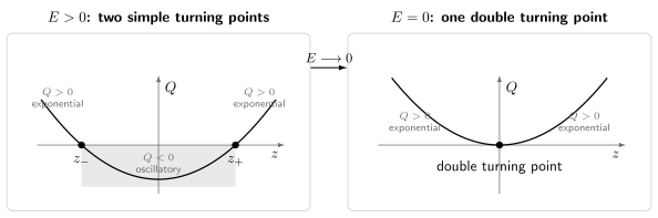
The Weber potential $Q(z)=z^2/4-E$ has two simple turning points for $E>0$; they merge at $E=0$. Along the real axis, solutions are oscillatory where $Q<0$ and exponential where $Q>0$.

When the $+$ turning point is well separated, choose $E^{1/6}$ compatibly with $\sqrt E$, so that $(E^{1/6})^3=\sqrt E$, and set

$$s = E^{1/6} \left( z-2\sqrt E \right).$$

On the same branches, direct substitution gives

$$\frac{\dd^2y}{\dd s^2} = \left[ s+\frac{s^2}{4E^{2/3}} \right]y.$$

Thus either separated Weber turning point has an Airy neighborhood, while the Weber equation retains both points in one global scaled model. The Airy approximation above is accurate on bounded $s$-sets as $|E|\to\infty$ in a fixed parameter sector; it is not uniform across both turning points.

The solution $D_\nu(z)$ is normalized by

$$D_\nu(z) \sim z^\nu\ee^{-z^2/4}, \qquad |\arg z| \leq \frac{3\pi}{4}-\delta,$$

uniformly on every such closed subsector, for fixed $\delta>0$, and on the chosen branch of $z^\nu$. The two formal exponential factors at infinity are $\ee^{-z^2/4}$ and $\ee^{z^2/4}$; infinity is an unramified irregular singularity of formal slope two, hence of minimal Poincaré rank two. Their equal-magnitude rays obey

$$\operatorname{Re}(z^2)=0, \qquad \arg z=\frac{\pi}{4}+\frac{k\pi}{2}.$$

This phase condition is safer than relying on inconsistent “Stokes” versus “anti-Stokes” terminology.

The right- and left-recessive solutions on the real line are

$$u_R(z,\nu)=D_\nu(z), \qquad u_L(z,\nu)=D_\nu(-z).$$

With the book’s Wronskian convention,

$$\Wr \left[ D_\nu(z), D_\nu(-z) \right] = \frac{\sqrt{2\pi}}{\Gamma(-\nu)}.$$

Consequently, the left-to-right boundary Wronskian is

$$F(\nu) = \Wr[u_L,u_R] = -\frac{\sqrt{2\pi}}{\Gamma(-\nu)}.$$

The sign records the ordering, while the zero set records when the two selected solution lines coincide.

For example, scale the harmonic oscillator

$$\left[ -\hbar^2\frac{\dd^2}{\dd x^2} + \alpha^2x^2 \right]\psi = \mathcal E\psi, \qquad \hbar,\alpha>0,$$

by

$$z=\sqrt{\frac{2\alpha}{\hbar}}\,x, \qquad \nu+\frac12 = \frac{\mathcal E}{2\alpha\hbar}.$$

Take the standard self-adjoint realization on $L^2(\mathbb R,\dd x)$ associated with the closed quadratic form

$$\begin{aligned} \mathfrak q[\psi] &= \int_{\mathbb R} \left( \hbar^2|\psi'(x)|^2 + \alpha^2x^2|\psi(x)|^2 \right)\dd x,\\ \mathcal D(\mathfrak q) &= H^1(\mathbb R) \cap L^2(\mathbb R,x^2\dd x). \end{aligned}$$

The scaling produces the displayed Weber equation. Square integrability at both real infinities is equivalent to the Wronskian condition

$$\frac1{\Gamma(-\nu)}=0.$$

Because gamma has poles at the nonpositive integers,

$$\nu=n\in\mathbb Z_{\ge0}, \qquad \mathcal E_n=(2n+1)\alpha\hbar.$$

At those values,

$$D_n(z) = 2^{-n/2} \ee^{-z^2/4} H_n\left( \frac{z}{\sqrt2} \right),$$

where $H_n$ is the physicists’ Hermite polynomial, and $D_n(-z)=(-1)^nD_n(z)$. Here an asymptotic connection Wronskian is also a spectral boundary function because the Hilbert space and self-adjoint realization have been declared.

More generally, consider an analytic parameter family whose potential has a nondegenerate double zero with a generic unfolding into two simple zeros. If no competing singularity lies nearby and the parameter remains in a fixed sector, a parameter-dependent Liouville transformation produces a Weber approximant with a controlled remainder across the pair. The quadratic Taylor model suggests the canonical equation; the transformation and remainder estimate establish uniformity. The exact harmonic oscillator is special because its reduction has no remainder.

Gauss resolves three regular singularities

The Gauss equation in this book is

$$z(1-z)y'' + \left[ c-(a+b+1)z \right]y' -ab\,y=0.$$

Its Riemann scheme is

$$P\!\left\{ \begin{matrix} 0&1&\infty\\ 0&0&a\\ 1-c&c-a-b&b \end{matrix} ;z \right\}.$$

The sum of all six exponents is

$$(1-c)+(c-a-b)+(a+b)=1,$$

the second-order Fuchs relation on the sphere. The exponent differences

$$\theta_0=1-c, \qquad \theta_1=c-a-b, \qquad \theta_\infty=a-b$$

are convenient gauge-invariant local parameters.

For this ordering of the exponent pairs, the inverse map is

$$\begin{aligned} c&=1-\theta_0,\\ a&= \frac{ 1-\theta_0-\theta_1+\theta_\infty }{2},\\ b&= \frac{ 1-\theta_0-\theta_1-\theta_\infty }{2}. \end{aligned}$$

Swapping the two exponents at a puncture flips the corresponding $\theta_j$. It can change the displayed $(a,b,c)$ even when the unordered local conjugacy data are unchanged.

Every second-order Fuchsian equation on the sphere with exactly three distinct singular points can be moved to $0,1,\infty$ by a Möbius transformation and reduced to this form by a scalar gauge. Once the three local exponent pairs are fixed, no accessory parameter remains. This is why the generic Gauss monodromy problem is rigid and why its connection coefficients reduce to gamma quotients.

The full normalized bases, lateral phases at infinity, gamma connection matrices, monodromy products, resonant limits, and Jacobi spectrum are worked out on the hypergeometric benchmark. The next page adds a fourth regular singular point. Its position supplies a cross-ratio and its coefficient data contain an accessory parameter, so local exponents no longer determine the global equation.

Exact equation or local approximation?

Before importing a special-function identity, classify the reduction:

Claim	What must be shown
Exact equivalence	An invertible coordinate and gauge transform the full equation, including all parameters
Leading local model	A scaled equation converges on a stated bounded scaled domain
Uniform approximation	The error is controlled across a turning-point or endpoint region
Formal normal form	Equality holds only as a formal asymptotic series
Spectral equivalence	The transform also maps the Hilbert space, domain, and boundary conditions

The distinction matters. A local Airy reduction predicts the transition through one turning point but does not by itself determine a two-end spectrum. A Weber reduction can be uniform across two merging turning points without making the original potential globally quadratic. A Liouville transform can preserve the solution space while changing its natural measure and endpoint domain.

A model-selection workflow

Given a new scalar equation:

1. Put it in Liouville normal form and retain the scalar gauge.
2. Locate poles and zeros of the normal-form coefficient.
3. Choose Airy for one simple zero, Bessel for an inverse-square endpoint, Weber for a quadratic well or coalescing pair, and Gauss for three regular singularities.
4. Derive the scaled variable instead of guessing it from notation.
5. Declare the exact local or asymptotic bases, their branches, and their sectors.
6. Check a Wronskian and one overlap, differential-equation, or monodromy identity.
7. Record resonant, polynomial, and degenerate parameter loci before taking limits.

This workflow selects the smallest model that retains the feature being studied. It also makes clear when the general or confluent Heun equation is genuinely needed.

The chapter route

Page	New question
Canonical Local Models	Which local geometry selects Airy, Bessel, Weber, or Gauss?
The General Heun Equation	How are the standard and normal forms normalized?
Accessory Parameters and Four-Point Geometry	What global freedom appears at four regular singularities?
The Confluence Hierarchy	How do HeunG, HeunC, HeunD, HeunB, and HeunT differ?
Canonical Local and Asymptotic Bases	Which basis belongs to each singular point or sector?
Möbius, Gauge, Discrete, and Confluence Transformations	Which operations preserve the equation class, and which are singular limits?
Parameter Crosswalks among Common Conventions	How do mathematical, physical, and software conventions translate?
Polynomial, Algebraic, and Quasi-Exactly Solvable Sectors	When do polynomial, algebraic, or quasi-exact solutions occur?

Common pitfalls

Calling a turning point singular. A zero of a normal-form potential is where a WKB basis fails, not necessarily where the exact ODE coefficients are singular. Airy’s finite turning point is ordinary.

Naming a function without its convention. Weber functions alone have several parameter conventions, and a symbol such as $U(a,z)$ is not the same parameterization as $D_\nu(z)$. State the differential equation first.

Dropping the scaling gauge. A coordinate change normally generates a first derivative. The compensating half-density affects Wronskians and boundary normalization.

Turning a local model into a global spectrum. Local decay or recessiveness becomes a spectral condition only after both endpoint conditions, the operator domain, and the parameter map have been supplied.

Exercises

1. Derive the Airy scale

Let

$$\hbar^2\psi''(z) = \left[ \kappa(z-z_0) + \beta(z-z_0)^2 \right]\psi(z), \qquad \kappa\neq0.$$

Find the scaled coordinate that makes the linear term exactly Airy, and determine the order of the quadratic correction for bounded scaled coordinate as $\hbar\to0$.

Solution

Set

$$\xi = \kappa^{1/3} \frac{z-z_0}{\hbar^{2/3}}, \qquad z-z_0 = \hbar^{2/3}\kappa^{-1/3}\xi.$$

Since

$$\frac{\dd^2}{\dd z^2} = \kappa^{2/3}\hbar^{-4/3} \frac{\dd^2}{\dd\xi^2},$$

division by $\kappa^{2/3}\hbar^{2/3}$ gives

$$\frac{\dd^2\psi}{\dd\xi^2} = \left[ \xi + \hbar^{2/3} \frac{\beta}{\kappa^{4/3}} \xi^2 \right]\psi.$$

Thus the correction is $O(\hbar^{2/3})$ on bounded $\xi$-sets. The branch of $\kappa^{1/3}$ fixes the rotation of the Airy sectors.

2. Audit the Bessel normal-form gauge

Starting from Bessel’s equation, set $u(z)=z^{1/2}y(z)$. Derive the normal-form equation and recover the exponents of $u$ at zero. For real $\nu\geq0$, determine when both local branches belong to $L^2((0,\varepsilon),\dd z)$.

Solution

The standard Liouville substitution for $y''+z^{-1}y'+(1-\nu^2z^{-2})y=0$ is $u=\exp(\tfrac12\int z^{-1}\dd z)y=z^{1/2}y$. Direct substitution gives

$$u'' + \left[ 1-\frac{\nu^2-\tfrac14}{z^2} \right]u =0.$$

Its indicial equation is

$$\rho(\rho-1) -\left( \nu^2-\frac14 \right) =0,$$

so

$$\rho_\pm=\frac12\pm\nu.$$

The shift by $1/2$ is exactly the exponent carried by the square-root gauge. For $\nu>0$ the two branches behave as $z^{1/2+\nu}$ and $z^{1/2-\nu}$. The first is always square-integrable, whereas the second is square-integrable exactly when

$$1-2\nu>-1, \qquad\text{that is,}\qquad \nu<1.$$

At $\nu=0$, both $z^{1/2}$ and the resonant branch $z^{1/2}\log z$ are square-integrable. Thus the endpoint is limit-circle for $0\leq\nu<1$ and limit-point for $\nu\geq1$.

3. Derive the Weber boundary Wronskian

Use

$$\begin{aligned} D_\nu(0) &= \frac{ 2^{\nu/2}\sqrt{\pi} }{ \Gamma\bigl((1-\nu)/2\bigr) },\\ D_\nu'(0) &= -\frac{ 2^{(\nu+1)/2}\sqrt{\pi} }{ \Gamma(-\nu/2) } \end{aligned}$$

to compute $\Wr[D_\nu(z),D_\nu(-z)]$. Then recover the two-sided oscillator quantization condition.

Solution

Because

$$\frac{\dd}{\dd z}D_\nu(-z) = -D_\nu'(-z),$$

evaluation at zero gives

$$\Wr \left[ D_\nu(z),D_\nu(-z) \right]_{z=0} = -2D_\nu(0)D_\nu'(0).$$

Substitution of the two special values and the duplication formula for gamma yield

$$\Wr \left[ D_\nu(z),D_\nu(-z) \right] = \frac{\sqrt{2\pi}}{\Gamma(-\nu)}.$$

The Wronskian is constant because the Weber equation has no first-derivative term. It vanishes precisely when $-\nu$ is a nonpositive integer:

$$\nu=n\in\mathbb Z_{\ge0}.$$

Using $\nu+\tfrac12=\mathcal E/(2\alpha\hbar)$ gives

$$\mathcal E_n=(2n+1)\alpha\hbar.$$

4. Resolve one Weber turning point

Let $E\neq0$ in $y''=(z^2/4-E)y$ and choose branches with $(E^{1/6})^3=\sqrt E$. Near $z_+=2\sqrt E$, set

$$s=E^{1/6}(z-z_+).$$

Derive the scaled equation and explain why this Airy reduction does not cover both turning points uniformly.

Solution

Write $z=2\sqrt E+E^{-1/6}s$. Then

$$\frac{z^2}{4}-E = E^{1/3}s + \frac14E^{-1/3}s^2,$$

while $\dd^2/\dd z^2=E^{1/3}\dd^2/\dd s^2$. Therefore

$$\frac{\dd^2y}{\dd s^2} = \left[ s+\frac{s^2}{4E^{2/3}} \right]y.$$

For bounded $s$ and large $|E|$ in a fixed parameter sector, the second term is small and the leading equation is Airy. The other turning point is at $z_-=-2\sqrt E$, whose distance from $z_+$ is $4\sqrt E$; it escapes to infinite $s$-distance in this local scaling. Weber, rather than one Airy chart, is the uniform model that retains the pair.

5. Check the Gauss exponent ledger

Derive the exponents of the Gauss equation at $0$, $1$, and $\infty$, and verify the Fuchs relation. Then reconstruct $(a,b,c)$ from

$$\left( \theta_0,\theta_1,\theta_\infty \right) = \left( \frac13,\frac14,\frac15 \right)$$

using the exponent ordering on this page.

Solution

At zero, substituting $y\sim z^\rho$ gives

$$\rho(\rho+c-1)=0,$$

so the exponents are $0$ and $1-c$. At one, put $t=1-z$ and obtain

$$\rho(\rho+a+b-c)=0,$$

so the exponents are $0$ and $c-a-b$.

At infinity, substitute $y\sim z^{-\rho}$. The leading balance gives

$$(\rho-a)(\rho-b)=0,$$

so the exponents in the local coordinate $1/z$ are $a$ and $b$. Their sum is

$$(1-c)+(c-a-b)+a+b=1,$$

as required for a second-order Fuchsian equation with three singular points on the sphere.

The inverse parameter map gives

$$\begin{aligned} c&=\frac23,\\ a&= \frac12 \left( 1-\frac13-\frac14+\frac15 \right) = \frac{37}{120},\\ b&= \frac12 \left( 1-\frac13-\frac14-\frac15 \right) = \frac{13}{120}. \end{aligned}$$

Here each prefactor $\tfrac12$ multiplies the following parenthesis. Reordering a local exponent pair flips the corresponding $\theta_j$ and therefore changes this displayed parameterization.

6. Show that the oscillator zeros are simple

Let

$$F(\nu) = -\frac{\sqrt{2\pi}}{\Gamma(-\nu)}.$$

Show that each zero $\nu=n\in\mathbb Z_{\geq0}$ is simple and compute $F'(n)$.

Solution

The residue of gamma at $z=-n$ is $(-1)^n/n!$, so

$$\Gamma(z) \sim \frac{(-1)^n}{n!(z+n)}.$$

Therefore

$$\frac1{\Gamma(-\nu)} \sim (-1)^{n+1}n!(\nu-n),$$

and hence

$$F'(n) = (-1)^n\sqrt{2\pi}\,n! \neq0.$$

The reciprocal-gamma quantization zeros are all simple. In operator language, this agrees with the simplicity of the one-dimensional harmonic oscillator spectrum.

7. Select the smallest adequate model

Choose the first canonical model to test in each situation:

1. one simple zero of $Q(z)$ in $\hbar^2y''=Qy$;

2. a radial endpoint satisfying

   $$u'' = \left[ \frac{\nu^2-\tfrac14}{r^2} + O(1) \right]u;$$

3. two turning points whose separation tends to zero;

4. four distinct regular singularities on the sphere.

Solution

1. Airy captures the simple turning point after an $\hbar^{2/3}$ scaling.
2. Bessel captures the inverse-square endpoint and its two Frobenius powers.
3. Weber is the uniform quadratic model for a coalescing pair.
4. None of the four models on this page is generically sufficient. Three regular singularities are Gauss-rigid, but the fourth introduces a cross-ratio and an accessory parameter. The general Heun equation is the next model.

In every case, “first model” means the smallest equation retaining the local or global datum of interest. Establishing an exact equivalence requires checking the full transformed equation, not only its leading singular term.

References

• NIST DLMF §9.2 and §9.7 give the Airy equation, Wronskians, connection formulae, and asymptotics; §2.8(iii), (vi) treats simple and coalescing turning points, and §12.16 develops parabolic-cylinder uniform approximations.
• NIST DLMF §10.2, §10.4, §10.5, and §10.8 give the Bessel definitions, connection identities, Wronskians, and logarithmic limiting cases; §10.17 gives the large-argument bases.
• NIST DLMF §12.2, §12.7, and §12.9 fix the parabolic-cylinder conventions, special values, Hermite specialization, and sectorial asymptotics; §2.7(ii) fixes the irregular-rank convention.
• NIST DLMF §18.39(i) gives the harmonic oscillator’s $L^2$ realization and spectrum; §1.18 reviews self-adjoint second-order differential operators and endpoint classification.
• NIST DLMF §15.10 gives the Gauss equation, local bases, and connection formulae; §15.11 gives the reduction of a three-singularity Fuchsian equation to Gauss form.
• NIST DLMF §31.2(i) identifies the singularity and accessory parameters of the four-point Heun equation.
• F. W. J. Olver, Asymptotics and Special Functions, A K Peters, 1997, develops turning-point transformations and uniform Airy and parabolic-cylinder approximations.
• N. M. Temme, Special Functions: An Introduction to the Classical Functions of Mathematical Physics, Wiley, 1996, provides a normalization-conscious account of the four model families.
• K. Iwasaki, H. Kimura, S. Shimomura, and M. Yoshida, From Gauss to Painlevé, Vieweg, 1991, develops the rigid three-point equation and the transition to accessory-parameter and monodromy-deformation problems.