Boundary Functions and Determinant Notions

Once an operator domain or radiation problem has been fixed, its admissible spectral parameters can often be detected by a scalar analytic function. That function may be a boundary value, a Wronskian, a determinant of solution frames, or an operator determinant. These constructions can have the same zeros in a particular problem without being the same object by definition.

This page separates four families of existence questions and then reconnects them by theorems. The first asks for analytic boundary modes, the second for a trace-ideal perturbation, the third for a spectral zeta series that converges in a right half-plane and continues regularly to zero, and the fourth for an entire function of controlled growth. A Dirichlet interval model will realize all four and expose the normalization constant that a bare zero set cannot determine.

Four constructions, four existence questions

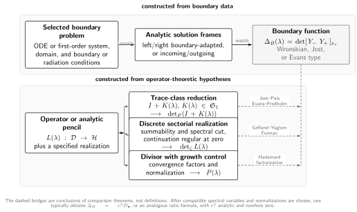
A boundary Wronskian or Jost–Evans function comes from a selected boundary problem, whereas Fredholm, zeta-regularized, and canonical-product determinants require distinct operator-theoretic hypotheses. The dashed bridges are comparison theorems, not definitional equalities.

The minimum data differ:

Construction	What must exist	What its zero or value means
Boundary Wronskian or Jost–Evans function	Analytic left and right solution subspaces with normalized frames	The selected subspaces intersect nontrivially
Fredholm determinant	A trace-class family $K(\lambda)$	$I+K(\lambda)$ is not invertible
Modified Fredholm determinant	A family in a stated Schatten class	The same invertibility test, with a different regularization
Zeta determinant	A spectral zeta series convergent in a right half-plane, a cut when needed, and regularity at zero	A regularized product attached to one operator
Canonical product	A discrete zero divisor and a convergence or growth estimate	An entire function with those zeros, still ambiguous by a zero-free factor

A finite-dimensional characteristic determinant is an ordinary determinant. Calling every other row “the determinant” suppresses precisely the hypotheses needed to know whether the object exists.

Boundary functions detect intersecting solution spaces

Consider the first-order system

$$Y'(x)=\mathcal A(x,\lambda)Y(x)$$

on $[a,b]$, and let its normalized propagator satisfy

$$\Phi(a,\lambda)=I.$$

Impose $n$ independent two-point conditions

$$C(\lambda)Y(a)+D(\lambda)Y(b)=0.$$

Every solution is $Y(x)=\Phi(x,\lambda)c$, so a nonzero solution satisfies the boundary conditions exactly when

$$\bigl[ C(\lambda)+D(\lambda)\Phi(b,\lambda) \bigr]c=0.$$

The characteristic boundary function

$$\Delta_B(\lambda) = \det\bigl[ C(\lambda)+D(\lambda)\Phi(b,\lambda) \bigr]$$

therefore vanishes precisely at characteristic values. If $\mathcal A$, $C$, and $D$ depend holomorphically on $\lambda$ under the usual uniform integrability assumptions, then so does $\Delta_B$. Premultiplying the boundary equations by an invertible analytic matrix $S(\lambda)$ changes the function to

$$\widetilde\Delta_B(\lambda) = \det S(\lambda)\,\Delta_B(\lambda).$$

The zero divisor is unchanged because $\det S$ is analytic and nowhere zero. Allowing a singular $S$ would add or remove zeros and would no longer be an innocuous change of boundary coordinates.

Assume $[C(\lambda)\ D(\lambda)]$ has constant rank $n$, and that the associated boundary pencil $T(\lambda)$ is a holomorphic Fredholm family of index zero for which the displayed characteristic matrix is a faithful finite-dimensional reduction. At an isolated characteristic value $\lambda_0$ of finite type,

$$\operatorname{ord}_{\lambda_0}\Delta_B = m_a(\lambda_0;T).$$

The nullity $\dim\ker T(\lambda_0)$ is only the geometric multiplicity, as explained on the preceding page.

Scalar Wronskians and Abel normalization

For

$$y''+p(x,\lambda)y'+q(x,\lambda)y=0,$$

let $y_L$ satisfy the selected left condition and $y_R$ the selected right condition. A common solution exists exactly when

$$\Wr[y_L,y_R](x,\lambda)=0.$$

Abel’s identity gives

$$\frac{\partial}{\partial x} \Wr[y_L,y_R] = -p(x,\lambda)\Wr[y_L,y_R].$$

After choosing a reference point $x_*$, the Abel-normalized function

$$\begin{aligned} E(\lambda) = \exp\left( \int_{x_*}^{x}p(s,\lambda)\,\dd s \right) \Wr[y_L,y_R](x,\lambda) \end{aligned}$$

is independent of $x$. In normal form, $p=0$ and the ordinary Wronskian is already constant.

If the boundary solutions are rescaled by analytic functions,

$$y_L\longmapsto a(\lambda)y_L, \qquad y_R\longmapsto b(\lambda)y_R,$$

then $E\mapsto abE$. The spectral zero divisor is preserved only when $a$ and $b$ are nowhere zero in the parameter region. This is why the leading coefficient, branch, and continuation path belong next to a Jost or boundary function.

Jost and Evans frames

For an $n$-component system on a noncompact interval, suppose an $r$-dimensional admissible subspace is selected at the left end and an $(n-r)$-dimensional one at the right. Choose analytic solution frames

$$Y_-(x,\lambda)\in\mathbb C^{n\times r}, \qquad Y_+(x,\lambda)\in\mathbb C^{n\times(n-r)}.$$

Their frame determinant is

$$d(x,\lambda) = \det\bigl( Y_-(x,\lambda)\ \ Y_+(x,\lambda) \bigr).$$

Liouville’s formula shows that

$$\begin{aligned} E_{\mathrm{Ev}}(\lambda) = \exp\left( -\int_{x_*}^{x} \operatorname{tr}\mathcal A(s,\lambda)\,\dd s \right) d(x,\lambda) \end{aligned}$$

is independent of the matching point. It vanishes exactly when the two admissible subspaces intersect.

Changing analytic frames by

$$Y_-\longmapsto Y_-G_-, \qquad Y_+\longmapsto Y_+G_+$$

multiplies $E_{\mathrm{Ev}}$ by $\det G_-\det G_+$. Hence an Evans function is naturally defined only up to a nowhere-vanishing analytic factor. Its construction also needs more than formal asymptotics: analytic exponential dichotomies, complementary dimensions, and analytic frames must exist in the parameter region. These hypotheses typically fail on essential spectrum or at a threshold.

A coordinate gauge $Y=G(x,\lambda)Z$ produces the precise covariance

$$E_{\mathrm{Ev}}^{(Y)}(\lambda) = \det G(x_*,\lambda)\, E_{\mathrm{Ev}}^{(Z)}(\lambda).$$

This follows because the frame determinant gains $\det G(x,\lambda)$ while the Liouville factor gains its reciprocal relative to $x_*$. On a parameter domain where the admissible subbundles are not globally trivial, one may need local Evans functions that glue as a section of a determinant line rather than one global scalar function.

For the Robin half-line model from the preceding page, the outgoing Jost solution is $f_+(x,k)=\ee^{\ii kx}$. The boundary functional gives

$$\begin{aligned} E_h(k) &= f_+'(0,k)-h f_+(0,k)\\ &= \ii k-h = \ii(k+\ii h). \end{aligned}$$

Its zero $k=-\ii h$ is exactly the pole of the continued Green kernel. For $h<0$ it is a physical-sheet eigenvalue; for $h>0$ it is a virtual pole on the lower half-plane. This boundary function is not thereby a Fredholm or zeta determinant. Such an identification needs another construction and a comparison theorem.

Fredholm determinants require a trace ideal

Let $K$ be trace class on a separable Hilbert space. Its Fredholm determinant can be defined by

$$\det_{\mathrm F}(I+K) = \sum_{j=0}^{\infty} \operatorname{tr}\bigl(\wedge^jK\bigr) = \prod_{n=1}^{\infty} \bigl(1+\nu_n(K)\bigr),$$

where $\{\nu_n(K)\}$ lists the nonzero eigenvalues with algebraic multiplicity. The sum and product converge absolutely, and

$$\det_{\mathrm F}(I+K)=0 \quad\Longleftrightarrow\quad I+K\ \text{is not invertible}.$$

When $\|K\|<1$, one also has

$$\log\det_{\mathrm F}(I+K) = \sum_{j=1}^{\infty} \frac{(-1)^{j+1}}{j} \operatorname{tr}(K^j).$$

The determinant itself extends beyond this small-norm disk. If $K(\lambda)$ is analytic in trace norm, then $\det_{\mathrm F}(I+K(\lambda))$ is analytic. At an isolated characteristic point of finite type, its zero order matches the characteristic multiplicity of the analytic Fredholm family.

Trace class is not a decorative assumption. If $K$ is Hilbert–Schmidt but not trace class, the ordinary product need not converge. The two-modified determinant is instead

$$\begin{aligned} \det{}_2(I+K) &= \det_{\mathrm F}\bigl((I+K)\ee^{-K}\bigr)\\ &= \prod_{n=1}^{\infty} \bigl(1+\nu_n(K)\bigr)\ee^{-\nu_n(K)}. \end{aligned}$$

For trace-class $K$,

$$\det{}_2(I+K) = \ee^{-\operatorname{tr}K} \det_{\mathrm F}(I+K).$$

Thus the ordinary and modified determinants have the same zeros but differ by a generally nonconstant zero-free factor. More generally, for an integer $p\ge2$ and $K\in\mathfrak S_p$,

$$\begin{aligned} \det{}_p(I+K) = \prod_{n=1}^{\infty} \bigl(1+\nu_n(K)\bigr) \exp\left[ \sum_{j=1}^{p-1} \frac{(-1)^j\nu_n(K)^j}{j} \right]. \end{aligned}$$

The regularization order is part of the notation. Modified determinants also need not be multiplicative; any correction factor must be tracked rather than inferred from finite-dimensional determinant rules.

The Birman–Schwinger bridge

Let $H=H_0+BA$ and take $z\in\rho(H_0)$. Under mapping hypotheses that make

$$K(z)=A(H_0-z)^{-1}B$$

a compact operator, the Birman–Schwinger principle identifies noninvertibility of $H-z$ with noninvertibility of $I+K(z)$. If $K(z)$ is trace class, this produces the perturbation determinant

$$D_{\mathrm F}(z) = \det_{\mathrm F}\bigl(I+K(z)\bigr).$$

If it is only Hilbert–Schmidt, $\det{}_2$ may be the available construction. The factorization, function spaces, and trace ideal must all be stated. This determinant is relative to $H_0$. Under the meromorphic Schatten-family hypotheses of the generalized Birman–Schwinger principle, the invariant at an isolated reference point is the operator-valued index

$$\begin{aligned} \operatorname{ind}_{C(z_0)}(I+K) &= \frac{1}{2\pi\ii} \operatorname{tr} \oint_{C(z_0)} \bigl(I+K(z)\bigr)^{-1} K'(z)\,\dd z\\ &= m_a(z_0;H)-m_a(z_0;H_0). \end{aligned}$$

Here $C(z_0)$ is a small positively oriented contour containing no other characteristic point.

Away from $\sigma(H_0)$, $K$ is analytic and the zero order of an available $\det{}_p(I+K)$ gives $m_a(z_0;H)$. At a reference eigenvalue, a meromorphic trace-class determinant may have an order equal to the displayed index, but for $p\ge2$ the modified determinant can instead have an essential singularity. The contour index, not an assumed zero-or-pole order, is the stable statement.

Where the inverses exist, the same factorization gives

$$\begin{aligned} (H-z)^{-1} = &(H_0-z)^{-1}\\ &- (H_0-z)^{-1}B \bigl(I+K(z)\bigr)^{-1} A(H_0-z)^{-1}. \end{aligned}$$

If the resolvent difference is trace class, differentiation of the Fredholm determinant yields

$$\frac{\dd}{\dd z} \log D_{\mathrm F}(z) = \operatorname{tr} \left[ (H_0-z)^{-1}-(H-z)^{-1} \right].$$

In one-dimensional scattering, Jost–Pais and later Evans-function comparison theorems identify a boundary function with a Fredholm or modified Fredholm determinant, sometimes only up to an explicit nowhere-vanishing factor. The equality follows from those theorems and their decay hypotheses—not from the word “determinant.”

Nor is every Fredholm determinant spectral. Isomonodromic tau functions can be represented by determinants of auxiliary contour or Plemelj operators built from a Riemann–Hilbert problem. Such a determinant belongs to the deformation problem; it is not the determinant of the original scalar ODE unless a separate theorem identifies the two operator constructions and their parameter constraints.

Zeta determinants need a summability half-plane

Let $A$ be a strictly positive self-adjoint operator with compact resolvent and positive eigenvalues $\{\mu_j\}$, counted with multiplicity. Assume in addition that $A^{-s_0}$ is trace class for some $s_0>0$. Then, initially for $\operatorname{Re}s>s_0$, its spectral zeta function is

$$\zeta_A(s) = \operatorname{tr}(A^{-s}) = \sum_j\mu_j^{-s}.$$

Suppose this function has a meromorphic continuation that is regular at $s=0$. The zeta-regularized determinant is

$$\det\nolimits_\zeta A = \exp\bigl(-\zeta_A'(0)\bigr).$$

Compact resolvent alone guarantees neither this summability half-plane nor the required continuation. Suitable regular elliptic realizations on compact manifolds or intervals acquire both from heat-kernel asymptotics. Regular-singular endpoints require separate choices of endpoint domain and separate heat- or resolvent-analysis theorems; regular interval formulas cannot simply be carried across the singular endpoint. For a nonnegative operator with a kernel, impose summability on the reduced inverse over $\ker(A)^\perp$; the primed determinant $\det'_\zeta A$ then omits the zero eigenvalues. For a nonselfadjoint sectorial operator, complex powers require a spectral cut; changing an admissible cut can change the answer.

Zeta regularization is not an ordinary infinite product. For $c>0$,

$$\det\nolimits_\zeta(cA) = c^{\zeta_A(0)} \det\nolimits_\zeta A.$$

The exponent $\zeta_A(0)$ is the regularized analogue of dimension. Likewise, finite-dimensional rules such as $\det(AB)=\det A\,\det B$ do not automatically survive: zeta determinants of elliptic operators can have a multiplicative anomaly.

For a parameter family $A-\lambda$, the defining formula applies directly only where the operator is invertible and a common cut is available. One may sometimes extend a normalized determinant across eigenvalues so that it vanishes there. Analyticity and multiplicity of that extension are theorems, not consequences of writing $\prod_j(\mu_j-\lambda)$.

Canonical products need zeros and growth

Suppose a discrete nonzero sequence $\{\lambda_j\}$ has no finite accumulation point. For an integer $p\ge0$, define the primary factors

$$\mathcal E_p(w) = (1-w) \exp\left( w+\frac{w^2}{2}+\cdots+\frac{w^p}{p} \right),$$

with $\mathcal E_0(w)=1-w$. If

$$\sum_j \frac1{|\lambda_j|^{p+1}} <\infty,$$

then

$$P(\lambda) = \lambda^m \prod_j \mathcal E_p\left( \frac{\lambda}{\lambda_j} \right)$$

converges locally uniformly and has exactly the prescribed zeros, including a zero of order $m$ at the origin. This is a canonical product.

The zeros do not determine an entire function. If $F$ has the same zero divisor as $P$, then

$$F(\lambda)=\ee^{g(\lambda)}P(\lambda)$$

for an entire function $g$. Finite-order growth can force $g$ to be a polynomial of bounded degree, while asymptotics and a value such as $F(0)$ may fix it further. Without those data, equality of spectra proves only equality up to a zero-free factor.

This construction also has a geometric scope. Resonances living on a logarithmic cover, a spectrum with finite accumulation, or a problem with branch cuts need not define an entire canonical product in the displayed spectral coordinate.

One interval problem realizes all four notions

Let

$$\begin{aligned} A_m&=-\frac{\dd^2}{\dd x^2}+m^2,\\ \mathcal D(A_m) &= H^2(0,L)\cap H_0^1(0,L), \qquad m>0. \end{aligned}$$

Its Dirichlet eigenvalues are

$$\mu_n = m^2+\left(\frac{n\pi}{L}\right)^2, \qquad n\ge1.$$

Consider $A_m+\alpha$ and let $u_\alpha$ solve

$$\begin{aligned} (A_m+\alpha)u_\alpha&=0,\\ u_\alpha(0)&=0, \qquad u_\alpha'(0)=1. \end{aligned}$$

Writing $\kappa^2=m^2+\alpha$ gives

$$u_\alpha(x) = \frac{\sinh(\kappa x)}{\kappa}.$$

Although $\kappa$ uses a square root, the quotient is an entire function of $\kappa^2$, hence of $\alpha$. Normalize the right boundary value at $\alpha=0$:

$$B_m(\alpha) = \frac{u_\alpha(L)}{u_0(L)} = \frac{ m\sinh(\kappa L) }{ \kappa\sinh(mL) }.$$

It vanishes exactly when

$$\alpha=-\mu_n, \qquad n\ge1,$$

so it is a normalized boundary function for loss of invertibility of $A_m+\alpha$.

The trace-class and product calculations

Because

$$\sum_{n=1}^{\infty}\frac1{\mu_n}<\infty,$$

$A_m^{-1}$ is trace class. Therefore

$$\begin{aligned} \det\nolimits_{\mathrm F} \bigl(I+\alpha A_m^{-1}\bigr) &= \prod_{n=1}^{\infty} \left( 1+\frac{\alpha}{\mu_n} \right). \end{aligned}$$

The product is genus zero. Euler’s product for $\sinh$ gives

$$\frac{\sinh(\kappa L)}{\kappa L} = \prod_{n=1}^{\infty} \left[ 1+\frac{\kappa^2L^2}{(n\pi)^2} \right].$$

Dividing this identity at $\kappa^2=m^2+\alpha$ by the identity at $\kappa=m$ yields

$$B_m(\alpha) = \prod_{n=1}^{\infty} \left( 1+\frac{\alpha}{\mu_n} \right) = \det\nolimits_{\mathrm F} \bigl(I+\alpha A_m^{-1}\bigr).$$

Euler’s product proves the exact equality. Their common value one at $\alpha=0$ fixes the remaining constant in this model.

The zeta calculation and its constant

The one-dimensional Gelfand–Yaglom theorem, in its zeta-determinant formulation for this Dirichlet problem, gives

$$\frac{ \det\nolimits_\zeta(A_m+\alpha) }{ \det\nolimits_\zeta A_m } = \frac{u_\alpha(L)}{u_0(L)} = B_m(\alpha)$$

where both sides are first taken on a common invertible region and then continued in $\alpha$. The absolute determinant is

$$\det\nolimits_\zeta A_m = \frac{2\sinh(mL)}{m}.$$

Consequently,

$$\begin{aligned} B_m(\alpha) &= \det\nolimits_{\mathrm F} \bigl(I+\alpha A_m^{-1}\bigr)\\ &= \frac{ \det\nolimits_\zeta(A_m+\alpha) }{ \det\nolimits_\zeta A_m }\\ &= \prod_{n=1}^{\infty} \left( 1+\frac{\alpha}{\mu_n} \right). \end{aligned}$$

This equality is the conclusion of trace-class, product, and Gelfand–Yaglom arguments. The unnormalized boundary value $u_\alpha(L)$ differs from the absolute zeta determinant by the factor $2$. The notation $\det_{\mathrm F}A_m$ is not defined: a Fredholm determinant applies to $I+T$ with $T$ trace class. What exists here is the relative determinant $\det_{\mathrm F}(I+\alpha A_m^{-1})$. The example therefore unifies the notions without erasing their definitions.

A determinant audit ledger

Before using a determinant-like function, record:

Datum	Question
Boundary problem	Which domain or radiation conditions are being detected?
Spectral coordinate	Is the function analytic in $\lambda$, $k$, $\lambda=k^2$, or only on a cover?
Solution normalization	Which leading coefficients, frames, branches, and matching point are fixed?
Operator class	Is the relevant operator finite rank, trace class, Hilbert–Schmidt, or merely compact?
Zeta data	Is the spectrum summable in a right half-plane, is a cut chosen, and is the zeta function regular at zero?
Product data	What is the exponent of convergence, genus, and zero-free factor?
Multiplicity	Is it a zero order, kernel dimension, contour index, or pole order?
Comparison theorem	Which result identifies two constructions, and what normalization remains?

The safest notation keeps the type visible: $E_{\mathrm{Ev}}$, $\det_{\mathrm F}$, $\det{}_2$, $\det_\zeta$, and $P$ should not be collapsed to a single $D$ until the comparison has been proved.

Common pitfalls

Calling a Wronskian a Fredholm determinant. A boundary Wronskian needs analytic solutions; a Fredholm determinant needs a trace-class reduction. They may agree in a scattering problem, but only under a comparison theorem.

Using a normalization with zeros. Multiplication by a nowhere-vanishing analytic factor preserves a characteristic divisor. A factor with a zero or pole changes the spectral count.

Writing an unregularized product of eigenvalues. Neither $\prod_j\mu_j$ nor $\prod_j(\mu_j-\lambda)$ usually converges. State whether the construction is Fredholm, zeta-regularized, or canonical.

Replacing $\det_{\mathrm F}$ by $\det{}_2$ silently. The modified determinant has the same zeros but differs by an exponential trace factor when both exist. That factor matters in derivative identities and absolute normalizations.

Equating entire functions from their zeros. A zero divisor determines an entire function only up to $\ee^{g(\lambda)}$. Growth and one or more normalization conditions are needed to determine $g$.

Ignoring cuts and zero modes. Zeta determinants of nonselfadjoint operators depend on an admissible spectral cut, while zero modes require a primed determinant or a parameter-dependent extension.

Exercises

1. Build a mixed-boundary function. For $-y''=\lambda y$ on $(0,L)$ with

$$y(0)=0, \qquad y'(L)+h\,y(L)=0,$$

normalize the left solution by $y'(0)=1$. Find an entire characteristic function of $\lambda$ and determine when $\lambda=0$ is an eigenvalue.

Solution

For $\lambda=k^2$, the normalized left solution is

$$y(x,\lambda) = \frac{\sin(kx)}{k},$$

with its value at $k=0$ understood by continuation. Applying the right boundary functional gives

$$\Delta_h(\lambda) = \cos(L\sqrt{\lambda}) +h\, \frac{\sin(L\sqrt{\lambda})}{\sqrt{\lambda}}.$$

Both terms have power series in integer powers of $\lambda$, so $\Delta_h$ is entire and independent of the choice of square-root branch. Its zeros are exactly the mixed-boundary eigenvalues. At zero,

$$\Delta_h(0)=1+hL.$$

Equivalently, the zero-energy solution is $y=x$, and its right condition is $1+hL=0$. Thus $\lambda=0$ is an eigenvalue precisely when $h=-1/L$.

2. Audit an analytic rescaling. Let a simple closed contour $\Gamma$ bound a domain $\Omega$, and let $E$ be holomorphic on a neighborhood of $\overline\Omega$ and nonzero on $\Gamma$. Compare its zero count in $\Omega$ with those of $\ee^{\lambda^2}E(\lambda)$ and $(\lambda-\lambda_0)E(\lambda)$, where $\lambda_0\in\Omega$ is not a zero of $E$.

Solution

The argument principle gives

$$N(E) = \frac1{2\pi\ii} \oint_\Gamma \frac{E'(\lambda)}{E(\lambda)} \,\dd\lambda.$$

For the first rescaling,

$$\frac{\dd}{\dd\lambda} \log\bigl(\ee^{\lambda^2}E\bigr) = 2\lambda+\frac{E'}E.$$

The integral of the entire function $2\lambda$ vanishes, so the zero count is unchanged. The second rescaling adds $1/(\lambda-\lambda_0)$ to the logarithmic derivative, whose contour integral is $2\pi\ii$. It therefore adds one zero. Only a nowhere-vanishing analytic normalization is spectrally harmless.

3. Match a point-interaction Jost function to a Fredholm determinant. Consider

$$H_\alpha = -\frac{\dd^2}{\dd x^2} +\alpha\delta_0$$

on the line. Use continuity at zero and

$$\psi'(0+)-\psi'(0-) = \alpha\psi(0)$$

to find the outgoing characteristic function. Then recover the same function from the rank-one Birman–Schwinger determinant and classify its zero for real $\alpha\ne0$.

Solution

Normalize the outgoing state to be

$$\psi(x) = \begin{cases} \ee^{-\ii kx},&x<0,\\ \ee^{+\ii kx},&x>0. \end{cases}$$

It is continuous at zero, while its derivative jump is $2\ii k$. The matching condition is therefore $2\ii k-\alpha=0$. Dividing by the free factor $2\ii k$ gives the Jost function

$$F_\alpha(k) = 1-\frac{\alpha}{2\ii k}.$$

For $\operatorname{Im}k>0$, the free resolvent kernel is

$$R_0(k^2;x,y) = \frac{\ii}{2k} \ee^{\ii k|x-y|}.$$

Interpreting the point interaction through its quadratic form and evaluation trace, the Birman–Schwinger auxiliary space is $\mathbb C$. Its operator is multiplication by $\alpha R_0(k^2;0,0)$, so its determinant is

$$1+\alpha R_0(k^2;0,0) = 1+\frac{\ii\alpha}{2k} = 1-\frac{\alpha}{2\ii k} = F_\alpha(k).$$

The zero is $k=-\ii\alpha/2$. For $\alpha<0$ it lies in the upper half-plane and gives the bound state of energy $-\alpha^2/4$. For $\alpha>0$ it lies on the lower continuation and is a virtual pole. The normalization and classification exclude the threshold $k=0$.

4. Use the determinant that actually exists. On $\ell^2(\mathbb N)$, let

$$K(z)e_n=\frac zn e_n.$$

Determine its Schatten class, construct its available determinant, and identify its zeros.

Solution

For $z\ne0$,

$$\sum_{n=1}^{\infty} \left|\frac zn\right|^2<\infty, \qquad \sum_{n=1}^{\infty} \left|\frac zn\right|=\infty.$$

Thus $K(z)\in\mathfrak S_2\setminus\mathfrak S_1$, so the ordinary Fredholm determinant is unavailable. The two-modified determinant is

$$\begin{aligned} \det{}_2(I+K(z)) &= \prod_{n=1}^{\infty} \left(1+\frac zn\right)\ee^{-z/n}\\ &= \frac{\ee^{-\gamma z}}{\Gamma(1+z)}, \end{aligned}$$

where $\gamma$ is Euler’s constant. It has simple zeros at $z=-1,-2,\ldots$, exactly where $I+K(z)$ is not invertible. The exponential factors remove the divergent linear terms that prevent the ordinary product from converging.

5. Differentiate the interval determinant. For the Dirichlet family $A_m+\alpha$, show that

$$\operatorname{tr}(A_m+\alpha)^{-1} = \frac{L}{2\kappa}\coth(\kappa L) -\frac1{2\kappa^2}, \qquad \kappa^2=m^2+\alpha,$$

away from its poles.

At $\kappa=0$, the right-hand side is understood by its removable limit

$$\frac{L^2}{6} = \operatorname{tr}A_0^{-1}.$$

Solution

The eigenvalue expansion gives

$$\operatorname{tr}(A_m+\alpha)^{-1} = \sum_{n=1}^{\infty} \frac1{\mu_n+\alpha}.$$

On the other hand,

$$\log B_m(\alpha) = \log\sinh(\kappa L)-\log\kappa+\text{constant},$$

and $\dd\kappa/\dd\alpha=1/(2\kappa)$. Hence

$$\frac{\dd}{\dd\alpha}\log B_m(\alpha) = \frac{L}{2\kappa}\coth(\kappa L) -\frac1{2\kappa^2}.$$

Differentiating either the Fredholm product or the zeta-determinant ratio gives

$$\frac{\dd}{\dd\alpha}\log B_m(\alpha) = \sum_{n=1}^{\infty} \frac1{\mu_n+\alpha},$$

which proves the identity. After filling in the removable point $\kappa=0$, the poles occur exactly when $A_m+\alpha$ is not invertible.

6. Fix the absolute zeta constant. Let $A_0=-\dd^2/\dd x^2$ with Dirichlet conditions on $(0,L)$. Compute $\det_\zeta A_0$ from the Riemann zeta values

$$\zeta_{\mathrm R}(0)=-\frac12, \qquad \zeta_{\mathrm R}'(0)=-\frac12\log(2\pi).$$

Solution

The eigenvalues are $(n\pi/L)^2$, so

$$\zeta_{A_0}(s) = \left(\frac{L}{\pi}\right)^{2s} \zeta_{\mathrm R}(2s).$$

Differentiation at zero gives

$$\begin{aligned} \zeta_{A_0}'(0) &= 2\log\left(\frac L\pi\right) \zeta_{\mathrm R}(0) +2\zeta_{\mathrm R}'(0)\\ &= -\log(2L). \end{aligned}$$

Therefore

$$\det\nolimits_\zeta A_0 = \exp\bigl(-\zeta_{A_0}'(0)\bigr) = 2L.$$

This is also the $m\to0$ limit of $2\sinh(mL)/m$.

7. Recover a function from zeros and growth. Suppose $F$ is entire of order at most $1/2$, has simple zeros exactly at $\lambda_n=(n\pi/L)^2$, and satisfies $F(0)=1$. Show that

$$F(\lambda) = \frac{\sin(L\sqrt{\lambda})}{L\sqrt{\lambda}}.$$

Solution

Since

$$\sum_{n=1}^{\infty}\frac1{\lambda_n}<\infty,$$

the zero sequence has a genus-zero canonical product

$$P(\lambda) = \prod_{n=1}^{\infty} \left( 1-\frac{\lambda}{\lambda_n} \right).$$

Hadamard factorization writes $F=\ee^Q P$, where the growth bound forces $Q$ to be a polynomial of degree at most zero. Thus $\ee^Q$ is constant, and $F(0)=P(0)=1$ fixes that constant to one. Euler’s sine product gives

$$P(\lambda) = \frac{\sin(L\sqrt{\lambda})}{L\sqrt{\lambda}},$$

whose apparent square-root branch is removable by its power series.

8. Name only the construction that exists. Identify what is justified in each case:

1. analytic outgoing modes exist, but no compact operator reduction is known;
2. a Birman–Schwinger family lies in $\mathfrak S_2$ but not $\mathfrak S_1$;
3. a positive elliptic realization has compact resolvent and a zeta function regular at zero;
4. resonance poles live only on a logarithmic cover of the energy plane.

Solution

In case 1 one may construct a Jost–Evans or boundary function, but no Fredholm determinant has been justified. In case 2 the available object is a two-modified Fredholm determinant, not the ordinary trace-class determinant. Case 3 supports a zeta determinant; it becomes a parameter-dependent characteristic function only after a family and continuation theorem are supplied. In case 4 the pole set does not by itself define an entire canonical product in the energy plane. A product might exist in another uniformizing coordinate, but that requires separate growth and convergence estimates.

References

• B. Simon, Trace Ideals and Their Applications, second edition, Mathematical Surveys and Monographs 120, AMS, 2005, for Schatten ideals, Fredholm determinants, and modified determinants.
• J. Behrndt, A. F. M. ter Elst, and F. Gesztesy, “The generalized Birman–Schwinger principle”, Transactions of the AMS 375 (2022), 799–845, for Jordan chains, analytic indices, and algebraic multiplicity in Birman–Schwinger families.
• J. Alexander, R. Gardner, and C. K. R. T. Jones, “A topological invariant arising in the stability analysis of travelling waves”, Journal für die reine und angewandte Mathematik 410 (1990), 167–212; see also B. Sandstede, “Stability of travelling waves”, Handbook of Dynamical Systems 2 (2002), 983–1055.
• F. Gesztesy, Y. Latushkin, and K. A. Makarov, “Evans functions, Jost functions, and Fredholm determinants”, Archive for Rational Mechanics and Analysis 186 (2007), 361–421, for exact and zero-free-factor comparisons with modified determinants.
• R. Jost and A. Pais, “On the scattering of a particle by a static potential”, Physical Review 82 (1951), 840–851, and B. Simon, “Resonances in one dimension and Fredholm determinants”, Journal of Functional Analysis 178 (2000), 396–420.
• K. Kirsten and A. J. McKane, “Functional determinants for general Sturm–Liouville problems”, Journal of Physics A 37 (2004), 4649–4670, for boundary-matrix formulas, arbitrary regular boundary conditions, and extracted zero modes.
• R. Forman, “Functional determinants and geometry”, Inventiones Mathematicae 88 (1987), 447–493, with erratum, for boundary reductions of zeta determinants.
• M. Lesch and B. Vertman, “Regular singular Sturm–Liouville operators and their zeta-determinants”, Journal of Functional Analysis 261 (2011), 408–450, for the additional domain and asymptotic analysis required at singular endpoints.
• L. Hartmann and M. Lesch, “Zeta and Fredholm determinants of self-adjoint operators”, Journal of Functional Analysis 283 (2022), 109491, for the exponential-polynomial correction relating zeta and modified Fredholm determinants.
• D. B. Ray and I. M. Singer, “R-torsion and the Laplacian on Riemannian manifolds”, Advances in Mathematics 7 (1971), 145–210, and R. T. Seeley, “Complex powers of an elliptic operator”, Proceedings of Symposia in Pure Mathematics 10 (1967), 288–307, for zeta regularization and spectral cuts.
• E. Elizalde, L. Vanzo, and S. Zerbini, “Zeta-function regularization, the multiplicative anomaly and the Wodzicki residue”, Communications in Mathematical Physics 194 (1998), 613–630, for multiplicative anomalies of zeta-regularized determinants.
• B. Ya. Levin, Distribution of Zeros of Entire Functions, Translations of Mathematical Monographs 5, AMS, 1964, for canonical products, exponent of convergence, and finite-order factorization.
• P. Gavrylenko and O. Lisovyy, “Fredholm determinant and Nekrasov sum representations of isomonodromic tau functions”, Communications in Mathematical Physics 363 (2018), 1–58, for the distinct auxiliary Fredholm determinants that represent isomonodromic tau functions.