Stage B: Canonical Sectorial Solutions and Local Connection Formulae

Page 3 divided the spatial surface into Stokes regions. A formal WKB branch in one such region is still not a canonical analytic solution. It becomes one only after the phase of $\hbar$, Borel direction, square-root sheet, normalization endpoint and path, spatial region, and lateral convention have all been fixed—and after the required summability theorem has been verified.

With those data in place, a simple turning point has a universal local answer. For a counterclockwise pair of adjacent regions, the turning-point-normalized bases are related by a unipotent triangular matrix whose nonzero off-diagonal entry is $+\ii$ in the source-facing relation. The matrix that replaces the continued source frame by the canonical destination frame is its inverse and contains $-\ii$. Rotated Airy functions fix this distinction exactly rather than mnemonically.

A simple pole is also a branch point of the WKB cover, but it is not an Airy turning point. In the standard meromorphic exact-WKB framework its multiplier is

$$2\ii\cos(\pi\nu_s), \qquad \nu_s^2=1+4b_s,$$

where $b_s$ is the double-pole coefficient of the $\hbar^2$ correction in Schrödinger normal form. This page derives the associated modified Bessel model, states the precise local theorem, and stops before the Voros transports and wall-crossing rules needed for global products.

Page question

Once a Stokes graph and Borel direction have been chosen, which data make a WKB solution canonical, and what are the correctly oriented local connection matrices at a simple zero or simple pole?

Status ledger

Statement used on this page	Status
Borel summation turns a formal WKB amplitude into an analytic solution	Theorem only under the stated coefficient, continuation, growth, path, and uniformity hypotheses
Regular-point exact WKB solution	Published existence and uniqueness theorem under complete-WKB-ray hypotheses
Turning-point normalization follows automatically from regular-point existence	False; the required limiting normalization is an additional issue
Ordered Wronskian $-2/\hbar$	Exact for the displayed unit-normalized pair when both sums use compatible normalization
Simple-zero triangular connection formula	Exact local theorem under the displayed summability and simple-turning-point hypotheses
Rotated-Airy calibration	Exact special-function identity and exact Wronskian calculation
Leading Langer map alone proves the universal exact multiplier	False; exact reduction and Borel summation supply the theorem
Simple-pole multiplier $2\ii\cos(\pi\nu_s)$	Exact theorem in the restricted meromorphic $R_0+\hbar^2R_2$ framework stated below
A product of bare local triangular matrices gives global monodromy	False unless every normalization transport, sheet relabelling, and singular-endpoint factor is included
Voros symbols and graph-wall mutations	Deferred to Page 5

“Canonical” is a data package, not a preferred formula

Retain the book’s normal form and Wronskian convention,

$$\begin{aligned} \hbar^2\psi'' &=R(z,\hbar)\psi, \\ R(z,\hbar) &=R_0(z)+O(\hbar), \\ \Wr[f,g] &=fg'-f'g, \\ \lambda_0 &=\sqrt{R_0(z)}\,\dd z. \end{aligned}$$

The word canonical will always be relative to a declared passport. At minimum it contains

$$\mathcal P = (\Theta_\hbar,L_\theta,D,\widehat z, N,\Gamma,\mathfrak s),$$

with the following meanings.

Datum	What it fixes
$\Theta_\hbar$	An $\hbar$-sector on which the summed solution is analytic
$L_\theta=\ee^{\ii\theta}\mathbb R_+$	The ray used by the book’s Borel–Laplace integral
$D$	A regular spatial Stokes region, or a smaller admissible domain inside it
$\widehat z\in\widehat\Sigma$	The square-root sheet and therefore the $+$/$-$ Riccati labels
$N$	A regular base point or a specified singular-endpoint normalization
$\Gamma$	The lifted continuation and integration path, including its homotopy class
$\mathfrak s$	Ordinary or lateral Borel prescription, with an explicitly oriented detour

Three uses of sector should not be conflated.

Sector-like object	Variable	Boundary selected by
Borel-summation sector	$\hbar$	Laplace decay and Borel growth
Stokes region	$z$	Critical horizontal trajectories of $\phi_\theta$
Canonical asymptotic sector at an irregular pole	$z$ near that pole	The local exponential asymptotics there

A solution can be sectorial in the first and third senses while being defined throughout one spatial Stokes region. None of these domains is a chamber in the parameter–phase space of Page 3.

Canonical does not mean global

Two authors can each define a canonical solution and obtain different connection constants because they chose different endpoints, sheets, paths, or scalar normalizations. The constants become comparable only after those data have been translated.

Borel summation supplies the analytic branches

Let

$$P_{\mathrm{even}} = \frac{P^{(+)}-P^{(-)}}{2}$$

be the branch-antisymmetric Riccati momentum of Chapter 8. When the potential is even in $\hbar$, its name also describes its literal parity. If odd powers occur, the same symbol still denotes the branch difference; it need not then be an even series.

For a regular base point or finite ramified endpoint $N$, and a lifted path $\Gamma_{N,z}$, the unit formal branches are

$$\begin{aligned} \widehat\psi_{\pm,N} ={}&P_{\mathrm{even}}(z,\hbar)^{-1/2} \\ &\times \exp\!\left[ \pm\frac{1}{\hbar} \int_{\Gamma_{N,z}} P_{\mathrm{even}}(\zeta,\hbar)\,\dd\zeta \right]. \end{aligned}$$

The infinite-pole analogue is defined only after the subtraction displayed below.

Factor the classical exponential before applying the ordinary shifted Borel transform of Page 1. For a regular or finite ramified endpoint, put

$$W_N(z) = \int_{\Gamma_{N,z}}\lambda_0,$$

with the half-contour interpretation when applicable. At an infinite pole, $W_N$ instead denotes the separately normalized classical primitive in the endpoint-subtracted formula below; the divergent integral from the pole is never used literally. In either case write

$$\widehat\psi_{\pm,N} = \exp\!\left(\pm\frac{W_N}{\hbar}\right) \widehat F_{\pm,N}.$$

Whenever $\widehat F_{\pm,N}$ is directionally summable with estimates locally uniform in $z\in D$, define

$$\begin{aligned} \Psi_{\pm,N}^{D,\theta}(z,\hbar) :={}& \exp\!\left(\pm\frac{W_N(z)}{\hbar}\right) \\ &\times \mathcal S_\theta \widehat F_{\pm,N}(z,\hbar). \end{aligned}$$

The Laplace kernel $\ee^{-\xi/\hbar}$ requires, more precisely, a subsector on which

$$\operatorname{Re} \left( \frac{\ee^{\ii\theta}}{\hbar} \right) >\kappa$$

for the applicable Borel growth rate $\kappa$. Thus the central choice $\arg\hbar=\theta$ is convenient but not part of the definition of the graph. Page 3’s graph angle and the actual $\hbar$ phase remain distinct data.

Under the analytic hypotheses of the summability theorem—rather than by formal coefficient matching alone—$\Psi_{\pm,N}^{D,\theta}$ solves the differential equation exactly. Nikolaev’s published theorem gives existence, uniqueness, and locally uniform Borel summation for the branch associated with one complete oriented WKB $(\theta,+)$ or $(\theta,-)$ ray, under its stated analyticity and uniformity assumptions. A two-solution basis needs the hypotheses for both rays, or the generic-strip setting of its Corollary 5.6. Classical saddle-free exact-WKB frameworks instead assemble admissible paths inside Stokes regions. These are complementary theorem packages, not a license to omit the hypotheses.

The normalization endpoint changes the object

A regular base point

If $b\in D$ is regular, a value-one formal normalization is

$$\begin{aligned} \widehat\chi_{\pm,b}(z,\hbar) ={}& \left[ \frac{P_{\mathrm{even}}(b,\hbar)} {P_{\mathrm{even}}(z,\hbar)} \right]^{1/2} \\ &\times \exp\!\left[ \pm\frac1\hbar \int_b^zP_{\mathrm{even}}\,\dd\zeta \right]. \end{aligned}$$

Then $\widehat\chi_{\pm,b}(b,\hbar)=1$. This pair differs from the unit WKB pair by a $z$-independent scalar on each branch. It is often best for an initial-value problem, but its local Stokes multiplier is not the bare Airy constant unless the normalization factors are also transported.

Its formal ordered Wronskian is correspondingly

$$\Wr[ \widehat\chi_{+,b}, \widehat\chi_{-,b} ] = -\frac{2}{\hbar} P_{\mathrm{even}}(b,\hbar).$$

For an analytic summed pair, the right-hand side must be interpreted through the same multiplicative summation prescription used to build the two solutions.

Existence of such a regular-point-normalized exact solution does not, by itself, establish the existence of a turning-point-normalized one. The normalization constant needed in the singular limit may fail to exist or fail to have the required asymptotics. This distinction is explicit in rigorous existence theory and should not be hidden by the same symbol $\Psi$.

A simple zero or simple pole

Let $e$ be an odd-order branch point of the spectral cover—a simple zero $a$ or, in the simple-pole framework below, a simple pole $s$. The formal coefficients are singular at the base endpoint, so $\int_e^zP_{\mathrm{even}}\,\dd z$ is not an ordinary improper integral and $\Psi(e)=1$ is not the normalization condition.

Choose the endpoint branch, a cut not crossing the Stokes edge in question, and a lifted contour $\gamma_z$ from $\tau(\widehat z)$ to $\widehat z$ that passes around the branch point with the prescribed orientation. Define coefficientwise

$$\int_e^z P_{\mathrm{even}}\,\dd\zeta := \frac12 \int_{\gamma_z} P_{\mathrm{even}}\,\dd\zeta.$$

Anti-invariance under the deck involution makes this the intrinsic turning-endpoint prescription. The half-contour also applies to the simple-pole branch point in Koike’s setting, with its local theorem and coefficient hypotheses. The direction in which $\gamma_z$ winds is part of the normalization.

A pole of order at least two

At an infinite pole $p$, the leading classical integral generally diverges. In the standard even framework one instead separates

$$\Omega(\hbar) = P_{\mathrm{even}}\,\dd z, \qquad \Omega^{\mathrm{reg}} = \Omega-\lambda_0,$$

and defines the regularized endpoint action and normalization by

$$\begin{aligned} \mathcal I_p(z) &:= \int_a^z\lambda_0 + \int_p^z\Omega^{\mathrm{reg}} , \\ \widehat\psi_{\pm,p} &= P_{\mathrm{even}}^{-1/2} \exp\!\left[ \pm\frac{\mathcal I_p(z)}{\hbar} \right]. \end{aligned}$$

Here the first term in $\mathcal I_p$ fixes a classical primitive through a chosen turning point $a$, while the second uses the endpoint-subtracted quantum form. Its existence depends on the pole-order and projective correction hypotheses reviewed in Chapter 8. More general irregular normalizations may require additional polynomial or logarithmic subtractions. None is a pointwise value at $p$.

Unit normalization makes the Wronskian a checksum

For the unit formal pair, direct differentiation gives

$$\Wr[ \widehat\psi_{+,N}, \widehat\psi_{-,N} ] = -\frac2\hbar.$$

When both amplitudes are summed compatibly and differentiation commutes with the Borel–Laplace integral, the analytic pair inherits the exact identity

$$\Wr[ \Psi_{+,N}^{D,\theta}, \Psi_{-,N}^{D,\theta} ] = -\frac2\hbar.$$

The traditional exact-WKB notation uses

$$S_{\mathrm{odd}}^{\mathrm{trad}} = \frac{P_{\mathrm{even}}}{\hbar}$$

and the prefactor $(S_{\mathrm{odd}}^{\mathrm{trad}})^{-1/2}$. Its solutions are $\sqrt\hbar$ times the book’s pair and therefore have ordered Wronskian $-2$. The common scalar does not alter a local connection matrix.

If two ordered frames $F_j=(f_{j,+},f_{j,-})$ satisfy

$$F_1=F_2C,$$

then

$$\det C = \frac{ \Wr[f_{1,+},f_{1,-}] }{ \Wr[f_{2,+},f_{2,-}] }.$$

Every local matrix below has determinant one. That test catches a surprising number of transpositions and normalization errors, though it cannot determine the sign of the off-diagonal entry.

Normal form matters

Wronskians are constant here because the equation has no first derivative. Before importing this ledger into $y''+p(z)y'+q(z)y=0$, either make the Liouville transformation or use Abel’s identity $W'=-pW$.

The oriented simple-zero theorem

Fix a Borel direction $\theta$ and its graph $G_\theta$ for $\phi_\theta=\ee^{-2\ii\theta}\phi_0$. Let $a$ be a simple zero, and let a Stokes edge $C$ issuing from $a$ separate adjacent regions $D_1$ and $D_2$. Make the following choices and assumptions:

1. $D_2$ is immediately counterclockwise from $D_1$ around $a$.
2. The branch cut used to label $\sqrt{R_0}$ does not cross $C$.
3. Both WKB branches use the same half-contour normalization at $a$.
4. The coefficient and geometric hypotheses required for Borel summability hold—for example, the saddle-free meromorphic framework of the theorem quoted in the references.
5. Analytic continuation is taken through a small regular point of $C$, not through the singular endpoint $a$.

One concrete theorem passport

Iwaki–Nakanishi I formulates this statement on a compact connected surface for a finite polynomial

$$R(z,\hbar) = \sum_{n=0}^{N}\hbar^nR_n(z)$$

with meromorphic coefficients. Its standing assumptions require at least one zero and one pole of $\phi_0$, all zeros simple, and no simple poles. Subleading poles occur only at poles of $\phi_0$. If $\phi_0$ has a pole of order $m\geq3$, then

$$\operatorname{ord}_pR_n < 1+\frac m2, \qquad n\geq1.$$

At a double pole, $R_n$ is at most simple for $n\geq1$ with $n\neq2$, while in a local coordinate $x$,

$$R_2(x) = -\frac{1}{4x^2}\bigl(1+O(x)\bigr).$$

The graph is assumed to have no recurrent trajectories and to be saddle-free for the displayed regional formula. If the surrounding quadratic differential has simple poles, Iwaki–Nakanishi II, Theorem 2.12, supplies the ordinary simple-zero connection formula in its more restrictive $R_0+\hbar^2R_2$ framework.

The local $+\ii$ theorem has published proofs through Voros and Aoki–Kawai–Takei. The regional summability statements quoted in Iwaki–Nakanishi I relied there on then-unpublished work of Koike–Schäfke. Page 3 records the provenance and a modern published summability theorem; the local formula here remains conditional on having the required sums.

On the chosen sheet define, along $C$ away from $a$,

$$\begin{aligned} w_{\theta,a}(z) &= \ee^{-\ii\theta} \int_a^z\lambda_0, \\ \varepsilon_C &:= \operatorname{sgn} \operatorname{Re}w_{\theta,a}(z). \end{aligned}$$

The real part is nonzero and has constant sign on the open edge. Put the scalar solutions into an ordered row frame

$$F_D = (\Psi_+^D,\Psi_-^D).$$

Write $F_{D_1}^{\to D_2}$ for the analytic continuation of the $D_1$ frame through a regular point of $C$ into $D_2$. In the component equations below, each left-hand $D_1$ solution is understood after that continuation.

For $\varepsilon_C=+1$, the source-facing connection formula is

$$\begin{aligned} \Psi_+^{D_1} &= \Psi_+^{D_2} +\ii\Psi_-^{D_2}, \\ \Psi_-^{D_1} &= \Psi_-^{D_2}. \end{aligned}$$

Equivalently,

$$F_{D_1}^{\to D_2} = F_{D_2}L(\ii), \qquad L(s) := \begin{pmatrix} 1&0\\ s&1 \end{pmatrix}.$$

For $\varepsilon_C=-1$,

$$\begin{aligned} \Psi_+^{D_1} &= \Psi_+^{D_2}, \\ \Psi_-^{D_1} &= \Psi_-^{D_2} +\ii\Psi_+^{D_2}, \end{aligned}$$

or

$$F_{D_1}^{\to D_2} = F_{D_2}U(\ii), \qquad U(s) := \begin{pmatrix} 1&s\\ 0&1 \end{pmatrix}.$$

These equations state the theorem in exactly the orientation printed in the standard source: the analytic continuation of the $D_1$ solution is re-expanded in the $D_2$ basis. If a transfer algorithm instead replaces that continued source frame by the canonical destination frame, it inverts the matrix:

$$F_{D_2} = F_{D_1}^{\to D_2} \begin{cases} L(-\ii),&\varepsilon_C=+1,\\ U(-\ii),&\varepsilon_C=-1. \end{cases}$$

Thus “counterclockwise gives $+\ii$” is incomplete. It gives $+\ii$ in $F_{D_1}^{\to D_2}=F_{D_2}C$ and $-\ii$ in the canonical-frame replacement $F_{D_2}=F_{D_1}^{\to D_2}C^{-1}$. Analytic continuation itself is encoded by the first relation, not by $C^{-1}$.

Rows of solutions are not columns of coefficients

The matrices above multiply a row frame on the right. If the two scalar basis functions are stacked into a column, transpose every displayed connection matrix. If a fixed analytic solution is expanded in the basis, its coefficient column transforms by the dual rule derived below.

What the triangular matrix actually changes

Dominant and subdominant branches

On the central $\hbar$ ray $\arg\hbar=\theta$,

$$\left| \frac{\Psi_+}{\Psi_-} \right| \asymp \exp\!\left[ \frac{2\operatorname{Re}w_{\theta,a}} {|\hbar|} \right].$$

When $\varepsilon_C=+1$, $\Psi_+$ is dominant and the theorem changes that basis element by a multiple of the unchanged subdominant one. For $\varepsilon_C=-1$, the roles are reversed. If $\vartheta=\arg\hbar\neq\theta$, actual magnitude is instead governed by

$$\operatorname{Re} \left[ \ee^{-\ii\vartheta}W_a(z) \right],$$

and on the edge this equals $\operatorname{Re}w_{\theta,a}\cos(\theta-\vartheta)$. Consequently the graph sign still agrees with dominance throughout the compatible Laplace half-plane $|\vartheta-\theta|<\pi/2$. It can reverse only after continuation beyond that half-plane; the formula above, not the central-ray mnemonic, remains the general test.

Coefficients of a fixed solution

Continue a fixed solution across $C$ and write its expansions before and after the crossing as

$$\psi=F_{D_j}c_j, \qquad c_j= \begin{pmatrix} A_j\\B_j \end{pmatrix}.$$

From $F_{D_1}^{\to D_2}=F_{D_2}C$ one obtains

$$c_2=Cc_1.$$

For $\varepsilon_C=+1$ this says

$$A_2=A_1, \qquad B_2=B_1+\ii A_1.$$

The dominant basis function changes, while the subdominant coefficient changes. Both familiar descriptions of the Stokes rule are therefore correct, but they refer to dual objects.

Sheet exchange and reversed crossing

The deck transformation exchanges the branch labels. With

$$J= \begin{pmatrix} 0&1\\1&0 \end{pmatrix},$$

one has

$$JL(\ii)J=U(\ii).$$

Reversing the spatial crossing gives

$$L(\ii)^{-1}=L(-\ii), \qquad U(\ii)^{-1}=U(-\ii).$$

Changing a sheet, reversing a path, transposing a basis convention, and inverting a crossing are four different operations. A sign table should record which one has actually been performed.

Scalar and endpoint renormalization

Suppose a new row frame is related to the endpoint-normalized one by

$$\widetilde F_D=F_DD_D,$$

where $D_D$ is diagonal and may itself be a Borel-summed open-action factor. Then

$$\widetilde F_{D_1} = \widetilde F_{D_2}\widetilde C, \qquad \widetilde C = D_{D_2}^{-1}CD_{D_1}.$$

If the same diagonal matrix $D$ is used on both sides,

$$\widetilde C=D^{-1}CD.$$

For example,

$$\begin{aligned} D &=\operatorname{diag}(d_+,d_-), \\ D^{-1}L(\ii)D &= \begin{pmatrix} 1&0\\ \ii d_+/d_-&1 \end{pmatrix}. \end{aligned}$$

The bare $\ii$ is therefore universal only in the local endpoint normalization. Regular-basepoint normalizations dress it by an open exponential, whose Borel sum and lateral behavior are Voros data.

Exact Airy functions fix the sign and scale

Consider the equation

$$\begin{aligned} \hbar^2\psi''&=z\psi, & \hbar&>0, \\ X&=\frac{z}{\hbar^{2/3}}, & \omega&=\ee^{2\pi\ii/3}. \end{aligned}$$

Take the positive Stokes edge, let $D_\downarrow$ lie just below it, and let $D_\uparrow$ lie just above it. Thus $D_\uparrow$ follows $D_\downarrow$ counterclockwise around the turning point. On the positive edge,

$$w_{0,0}(z) = \frac23z^{3/2}>0,$$

so the growing branch is labelled $+$ and the recessive branch is labelled $-$. Define the exact solutions

$$\begin{aligned} A(z,\hbar) &= 2\sqrt\pi\,\hbar^{-1/6}\Ai(X), \\ G_\downarrow(z,\hbar) &= 2\sqrt\pi\,\hbar^{-1/6} \ee^{\ii\pi/6}\Ai(\omega X), \\ G_\uparrow(z,\hbar) &= 2\sqrt\pi\,\hbar^{-1/6} \ee^{-\ii\pi/6}\Ai(\omega^2X). \end{aligned}$$

Equivalently,

$$\begin{aligned} G_\downarrow &= \sqrt\pi\,\hbar^{-1/6} \bigl[\Bi(X)+\ii\Ai(X)\bigr], \\ G_\uparrow &= \sqrt\pi\,\hbar^{-1/6} \bigl[\Bi(X)-\ii\Ai(X)\bigr]. \end{aligned}$$

The sectorial Airy asymptotics give precisely the book’s unit leading WKB amplitudes:

$$\begin{aligned} A &\sim z^{-1/4} \exp\!\left(-\frac{2z^{3/2}}{3\hbar}\right), \\ G_{\downarrow,\uparrow} &\sim z^{-1/4} \exp\!\left(+\frac{2z^{3/2}}{3\hbar}\right) \end{aligned}$$

on their respective sides of the ray. The exact rotated-Airy identity

$$\Ai(X) +\omega^2\Ai(\omega^2X) +\omega\Ai(\omega X) =0$$

is equivalent to

$$G_\downarrow = G_\uparrow+\ii A.$$

Therefore

$$(G_\downarrow,A) = (G_\uparrow,A)L(\ii),$$

which is exactly the $\varepsilon_C=+1$ theorem with $D_1=D_\downarrow$ and $D_2=D_\uparrow$. Solving instead for the canonical upper basis gives the replacement rule

$$(G_\uparrow,A) = (G_\downarrow,A)L(-\ii).$$

The Wronskian fixes the remaining normalization. Since $\partial_z=\hbar^{-2/3}\partial_X$ and $\Wr_X[\Ai,\Bi]=1/\pi$,

$$\Wr_z[G_\downarrow,A] = \Wr_z[G_\uparrow,A] = -\frac2\hbar.$$

This one model simultaneously calibrates the side ordering, row-frame convention, $+\ii$ in the analytic-continuation relation, $-\ii$ in the canonical-frame replacement, and the book’s $-2/\hbar$ Wronskian.

One circuit is not three matrices equal to the identity

Successive canonical-frame replacements around the three Airy edges alternate lower and upper inverse shears. Their product is

$$L(-\ii)U(-\ii)L(-\ii) = \begin{pmatrix} 0&-\ii\\ -\ii&0 \end{pmatrix} = -\ii J.$$

This is not a contradiction with the fact that Airy functions are entire. A circuit around the simple branch point also sends

$$\sqrt{R_0}\longmapsto-\sqrt{R_0}, \qquad R_0^{-1/4}\longmapsto-\ii R_0^{-1/4},$$

and hence relabels the formal WKB frame by the same matrix $-\ii J$. The analytic local monodromy is trivial only after this formal sheet and prefactor transport is included:

$$L(-\ii)U(-\ii)L(-\ii)(-\ii J)^{-1}=I.$$

The Langer coordinate explains universality, but does not prove it

Near a general simple zero $a$, choose a sheet and set

$$\zeta(z) = \left[ \frac32 \int_a^z\sqrt{R_0(t)}\,\dd t \right]^{2/3}.$$

Then

$$\zeta(\zeta')^2=R_0.$$

With

$$\psi(z) = (\zeta'(z))^{-1/2}Y(\zeta),$$

the transformed equation is

$$\hbar^2Y_{\zeta\zeta} = \left[ \frac{R(z,\hbar)}{(\zeta')^2} + \frac{\hbar^2}{2(\zeta')^2} \{\zeta,z\} \right]Y,$$

where

$$\{\zeta,z\} = \frac{\zeta'''}{\zeta'} -\frac32 \left(\frac{\zeta''}{\zeta'}\right)^2$$

is the Schwarzian derivative. Its leading term is the Airy equation $\hbar^2Y_{\zeta\zeta}=\zeta Y$. For the exactly linear potential $R_0=c(z-a)$, the scaled variable

$$X = \frac{c^{1/3}(z-a)}{\hbar^{2/3}}$$

reduces the equation to Airy exactly, and all three unit-normalized solutions acquire the common factor $c^{-1/6}$.

For a nonlinear $R_0$ or a nonzero subleading potential, the Schwarzian and subleading terms remain. The universal multiplier then follows from the exact local transformation and Borel analysis in the connection theorem—not from discarding those corrections in a leading Airy approximation.

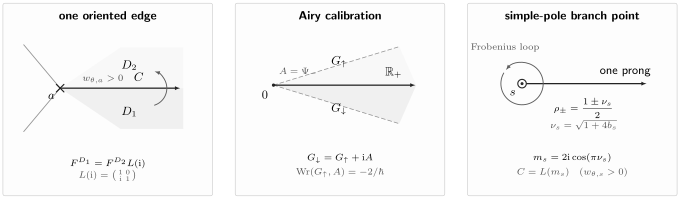
Local connection passport. Left: $D_2$ follows $D_1$ counterclockwise, so the analytically continued source frame obeys $F_{D_1}^{\to D_2}=F_{D_2}L(\ii)$; the figure abbreviates the continuation superscript. Center: rotated Airy functions fix that sign and the ordered Wronskian exactly. Right: a simple-pole branch point has one prong and remembers the Frobenius exponent difference $\nu_s$, replacing $\ii$ by $2\ii\cos(\pi\nu_s)$.

A simple-pole branch point is a different local problem

The Airy formula applies to a simple zero of $R_0$. A simple pole of the leading quadratic differential is also a ramification point of the spectral cover and emits one Stokes prong, but its exact local connection remembers subleading regular-singular data.

Use the restricted meromorphic framework

$$R(z,\hbar) = R_0(z)+\hbar^2R_2(z).$$

Near a simple pole $s$, in a local Schrödinger coordinate, write

$$\begin{aligned} R_0(z) &= \frac{a_s}{z-s}+O(1), \\ R_2(z) &= \frac{b_s}{(z-s)^2} +O\!\left((z-s)^{-1}\right). \end{aligned}$$

Define

$$\begin{aligned} \nu_s &= \sqrt{1+4b_s}, \\ t_s &= \ee^{\pi\ii\nu_s}, \\ \kappa_s &= t_s+t_s^{-1} = 2\cos(\pi\nu_s), \\ m_s &= \ii\kappa_s = 2\ii\cos(\pi\nu_s). \end{aligned}$$

This notation separates the symmetric trace-like quantity $\kappa_s$ from the full off-diagonal multiplier $m_s$.

Simple-pole hypotheses

The global framework used here assumes a compact connected surface and meromorphic $R_0,R_2$. The quadratic differential $\phi_0$ has at least one zero and one pole, and all its zeros are simple. Poles of $R_2$ occur only at poles of $\phi_0$, with the following local requirements.

• At a simple pole $s$, $\operatorname{ord}_sR_2\leq2$.
• At a double pole $p$, in an appropriate local coordinate $x$, $R_2(x)=-(4x^2)^{-1}\bigl(1+O(x)\bigr)$.
• At a pole $p$ of order $m\geq3$, $\operatorname{ord}_pR_2<1+m/2$.

The trajectory foliation has no recurrent leaves, and the graph is saddle-free for the displayed summed connection formula. The result is not asserted here for an arbitrary $\hbar R_1$, arbitrary higher $\hbar$-dependence, a higher-order zero, or coalescing critical points.

Normalize both branches at $s$ by the contour prescription described above. With the same region ordering and sign $\varepsilon_C=\operatorname{sgn}\operatorname{Re}w_{\theta,s}$, the simple-pole connection theorem is

$$F_{D_1} = F_{D_2} \begin{cases} L(m_s),&\varepsilon_C=+1,\\ U(m_s),&\varepsilon_C=-1. \end{cases}$$

Replacing the continued $D_1$ frame by the canonical $D_2$ frame again uses the inverse and hence $-m_s$. The theorem imposes no extra nonresonance condition on $\nu_s$; the formula is invariant under $\nu_s\mapsto-\nu_s$. At

$$\nu_s\in\mathbb Z+\frac12,$$

the multiplier vanishes even though the geometric one-prong edge remains.

The modified-Bessel model exposes the exponent difference

Take the exactly solvable model

$$\begin{aligned} \hbar^2\psi'' &= \left( \frac{a}{x} + \frac{\hbar^2b}{x^2} \right)\psi, \\ a&>0, &x&>0, &\hbar&>0. \end{aligned}$$

Set

$$\begin{aligned} X&=\frac{2\sqrt{ax}}{\hbar}, \\ \psi(x)&=\sqrt{x}\,u(X), \\ \nu^2&=1+4b. \end{aligned}$$

Direct substitution gives the modified-Bessel equation

$$X^2u_{XX} +Xu_X -(X^2+\nu^2)u =0.$$

The exact pair

$$\begin{aligned} \Psi_+^{I} &= 2\sqrt{\frac{\pi}{\hbar}}\, \sqrt{x}\,I_\nu(X), \\ \Psi_-^{K} &= \frac{2}{\sqrt{\pi\hbar}}\, \sqrt{x}\,K_\nu(X) \end{aligned}$$

has the unit WKB leading behavior

$$\Psi_\pm \sim \left(\frac{a}{x}\right)^{-1/4} \ee^{\pm X}$$

and, using $\Wr_X[K_\nu,I_\nu]=1/X$,

$$\Wr_x[\Psi_+^{I},\Psi_-^{K}] = -\frac2\hbar.$$

Two continuations of the growing solution across the relevant cut can be normalized as

$$\begin{aligned} G_\downarrow &= \frac{2\ii}{\sqrt{\pi\hbar}}\, \sqrt{x}\, K_\nu(\ee^{\pi\ii}X), \\ G_\uparrow &= -\frac{2\ii}{\sqrt{\pi\hbar}}\, \sqrt{x}\, K_\nu(\ee^{-\pi\ii}X). \end{aligned}$$

For $X>0$, the standard continuation identities

$$\begin{aligned} K_\nu(\ee^{\pi\ii}X) &= \ee^{-\pi\ii\nu}K_\nu(X) -\pi\ii I_\nu(X), \\ K_\nu(\ee^{-\pi\ii}X) &= \ee^{\pi\ii\nu}K_\nu(X) +\pi\ii I_\nu(X) \end{aligned}$$

give

$$G_\downarrow-G_\uparrow = 2\ii\cos(\pi\nu)\,\Psi_-^{K}.$$

Moreover,

$$\Wr_x[G_\downarrow,\Psi_-^{K}] = \Wr_x[G_\uparrow,\Psi_-^{K}] = -\frac2\hbar.$$

The model thus reproduces both the Koike multiplier and its unit-normalized Wronskian. The theorem for a general admissible simple pole additionally requires the exact local reduction and summability argument.

The multiplier is local monodromy data

Near $x=0$, the indicial equation is

$$\rho(\rho-1)=b.$$

Thus

$$\rho_\pm = \frac{1\pm\nu}{2}, \qquad \ee^{2\pi\ii\rho_\pm} = -\ee^{\pm\pi\ii\nu}.$$

If $M_s$ denotes the local Frobenius monodromy, then

$$\operatorname{tr}M_s = -2\cos(\pi\nu), \qquad m_s = -\ii\,\operatorname{tr}M_s.$$

At resonant integer $\nu$, the trace formula remains valid even when a logarithm makes the monodromy nondiagonalizable. The connection multiplier depends on the exponent difference, or equivalently on $b_s$. It does not depend on $a_s$, and it is not a residue of $\lambda_0$: on the spectral cover, $\lambda_0$ is regular and nonzero above a simple pole.

Compute $b_s$ only after putting the equation into Schrödinger, or projective, normal form. A first-derivative removal contributes to the double-pole coefficient and can therefore change $\nu_s$.

Spatial crossing and lateral summation are related, not identical

The local theorem above fixes $\theta$ and compares two spatial regions. Both regional solutions use the same Borel ray:

$$D_1\longleftrightarrow D_2, \qquad \text{$z$ varies, $L_\theta$ fixed}.$$

A lateral Stokes discontinuity instead fixes a regular spatial point and compares rays immediately above and below a singular Borel direction:

$$\mathcal S_{\theta+} \longleftrightarrow \mathcal S_{\theta-}.$$

Here $z$ is fixed and the Borel contour varies.

The book uses $+$ for the contour above the oriented Borel ray and $-$ for the contour below it. Fix a small $\epsilon>0$. For a simple-zero edge, assume that every graph throughout the closed phase interval $[\theta-\epsilon,\theta+\epsilon]$ is saddle-free, and that the fixed spatial point lies on the graph only at the central phase $\theta$. Let $F_{\theta+}$ and $F_{\theta-}$ denote the two lateral sums of the same endpoint-normalized formal row frame at that point, with the sheet, lifted normalization path, and branch labels held fixed. The phase-rotation form of the ordinary connection theorem then translates to

$$F_{\theta+} = F_{\theta-} \begin{cases} L(\ii),&\varepsilon_C=+1,\\ U(\ii),&\varepsilon_C=-1. \end{cases}$$

This equality is the translated simple-zero corollary, with its own uniformity hypotheses; it is not the definition of the spatial connection. A simple-pole analogue would replace $\ii$ by $m_s$ and requires the restricted simple-pole framework and a uniformly controlled graph family. It is not being folded into the displayed ordinary formula. In particular, the $+$/$-$ notation in Iwaki–Nakanishi’s later wall-crossing sections is opposite to this book’s above/below convention after $\arg\eta=-\arg\hbar$ is translated. Importing only the symbols would reverse the jump.

Keep these five operations distinct.

• Continue and re-expand. Keep the Borel ray $L_\theta$ fixed, change the spatial region, and use $F_{D_1}^{\to D_2}=F_{D_2}C$.
• Replace by the destination frame. Keep the continued solution space fixed, change the canonical basis, and use $F_{D_2}=F_{D_1}^{\to D_2}C^{-1}$.
• Compare lateral Borel sums. Keep a regular $z$ fixed, move the contour above or below $L_\theta$, and invoke the translated lateral theorem.
• Exchange sheets. Keep the base point $z$ fixed, change its lift on $\widehat\Sigma$, conjugate by $J$, and relabel the signs.
• Reverse a path. Keep its endpoints, reverse its orientation, and invert the associated transport.

Local matrices need diagonal transport before they become global

Suppose $\beta$ is an oriented lifted path from a ramified endpoint $a$ to another ramified endpoint $b$, and define the closed anti-invariant cycle

$$\gamma = \beta-\tau_*\beta.$$

With the orientation just declared,

$$\oint_\gamma P_{\mathrm{even}}\,\dd z = 2\int_a^b P_{\mathrm{even}}\,\dd z.$$

Introduce the total formal Voros exponent

$$\widehat V_\gamma^{\mathrm{tot}} := \frac1\hbar \oint_\gamma P_{\mathrm{even}}\,\dd z.$$

The two endpoint-normalized formal frames satisfy

$$\widehat F_a = \widehat F_b \begin{pmatrix} \exp(\widehat V_\gamma^{\mathrm{tot}}/2)&0\\ 0&\exp(-\widehat V_\gamma^{\mathrm{tot}}/2) \end{pmatrix}.$$

This identity is formal until the open or closed exponent is regularized and Borel-summed with its complete path and lateral passport. If a route crosses an edge emitted by $b$ while the current frame is normalized at $a$, the bare $L(\ii)$ or $U(\ii)$ must be conjugated by this diagonal transport. At a simple pole, replace the local $\ii$ by $m_s$ but keep the same normalization logic.

A single edge therefore contributes a universal local shear. A global connection calculation alternates such shears with diagonal open-path transports, branch-cut relabellings, formal monodromy factors, and possibly singular-endpoint matrices. Page 5 constructs the required Voros symbols and derives how their Borel sums change when a saddle wall is crossed.

A reliable local-connection workflow

For a concrete equation, use the following order.

1. Put the equation in Schrödinger normal form and record how the dependent variable changed.
2. Fix $\theta$, the compatible $\hbar$-sector, the phased quadratic differential, and a square-root sheet.
3. Construct the Stokes graph and verify the summability hypotheses on the regions and paths actually used.
4. Classify the emitting critical point: simple zero, simple pole, higher-order zero, or another singularity.
5. Draw the cut away from the selected edge and specify the endpoint half-contour or pole subtraction.
6. Order $D_1,D_2$ counterclockwise and compute $\varepsilon_C=\operatorname{sgn}\operatorname{Re}w_{\theta,e}$.
7. Write the source-facing matrix $F_{D_1}^{\to D_2}=F_{D_2}C$. Invert it only when replacing the continued source frame by the canonical destination frame.
8. Conjugate by any change of endpoint or scalar normalization.
9. Check the determinant and ordered Wronskian.
10. Multiply local and transport factors in path order, keeping sheet relabellings explicit.

This workflow is deliberately more verbose than the mnemonic “dominant picks up subdominant.” The extra ledger is what makes the answer reproducible.

Reproducible checks

The companion script audits the convention-sensitive algebra and the two exactly solvable models. It verifies:

• Airy scaling, rotated identities, unit amplitudes, and the $-2/\hbar$ Wronskians;
• the lower and upper triangular matrices, their inverses, determinant, sheet conjugation, and three-edge closure;
• diagonal normalization conjugation;
• the simple-pole substitution into the modified-Bessel equation;
• the normalized $I_\nu$–$K_\nu$ Wronskian and two continuation identities;
• the multiplier $2\ii\cos(\pi\nu)$, its branch invariance, and its half-integer zeros.

Download the canonical-sectorial connection checker

Run it from the project root:

python3 public/code/advanced-ode/canonical-sectorial-connection-check.py

The script checks identities and representative high-precision special-function values. It does not prove Borel summability, the general exact reduction theorem, or a global monodromy formula.

Common pitfalls

Calling a branch canonical without its passport. A formal sign is not a canonical analytic solution. Record the $\hbar$-sector, Borel ray, spatial region, sheet, endpoint, path, lateral prescription, and scalar normalization.

Treating a ramified endpoint as an initial value. The formula $\int_a^zP_{\mathrm{even}}\dd z$ at a simple zero or simple pole is a half-contour on the cover. It does not mean that the singular formal expression has been evaluated at $a$.

Mixing a row basis with a coefficient column. Right multiplication changes basis functions, whereas the coefficients of a fixed solution obey the dual relation. Transposing one convention without transposing the other changes which entry jumps.

Calling $\ii$ basis-independent. It is universal in the declared unit endpoint normalization. A diagonal change of normalization conjugates the triangular matrix and dresses its off-diagonal entry.

Applying Airy at a simple pole. A simple pole has one prong, not three, and its exact multiplier depends on the Frobenius exponent difference. The ordinary Airy formula also does not cover a higher-order or merging turning point.

Computing the pole parameter before removing the first derivative. The Liouville transformation can alter the double-pole coefficient. Koike’s $b_s$ belongs to Schrödinger normal form.

Demanding identity from three bare Airy shears. A circuit also exchanges sheets and rotates the fourth-root prefactor. The product of the three canonical-frame replacement shears is $-\ii J$, exactly the missing formal-frame transport.

Multiplying local matrices with incompatible endpoints. The bare Airy and simple-pole constants assume normalization at the edge’s emitting critical point. Changing that endpoint inserts a diagonal Voros transport before the next local shear.

Exercises

1. Read the two matrix conventions

Expand

$$F_1=F_2L(\kappa), \qquad F_1=F_2U(\kappa)$$

into component relations. Derive the inverse canonical-frame replacement rules and the coefficient transformation for a fixed solution.

Solution

For $F_j=(\Psi_+^j,\Psi_-^j)$,

$$F_1=F_2L(\kappa)$$

means

$$\Psi_+^1 = \Psi_+^2+\kappa\Psi_-^2, \qquad \Psi_-^1 = \Psi_-^2.$$

Similarly,

$$F_1=F_2U(\kappa)$$

means

$$\Psi_+^1 = \Psi_+^2, \qquad \Psi_-^1 = \Psi_-^2+\kappa\Psi_+^2.$$

Because

$$L(\kappa)^{-1}=L(-\kappa), \qquad U(\kappa)^{-1}=U(-\kappa),$$

write $F_1^{\to2}$ for the continued source frame. The two canonical-frame replacements are

$$F_2 = F_1^{\to2}L(-\kappa), \qquad F_2 = F_1^{\to2}U(-\kappa).$$

If $\psi=F_jc_j$ is fixed and $F_1^{\to2}=F_2C$, then

$$c_2=Cc_1.$$

Thus for a lower shear,

$$\begin{aligned} A_2&=A_1, \\ B_2&=B_1+\kappa A_1. \end{aligned}$$

For an upper shear,

$$\begin{aligned} A_2&=A_1+\kappa B_1, \\ B_2&=B_1. \end{aligned}$$

2. Recover every Airy normalization constant

Starting from

$$\begin{aligned} \Ai(X) &\sim \frac{X^{-1/4}}{2\sqrt\pi} \ee^{-2X^{3/2}/3}, \\ \Bi(X) &\sim \frac{X^{-1/4}}{\sqrt\pi} \ee^{2X^{3/2}/3}. \end{aligned}$$

derive the factors in $A$, $G_\downarrow$, and $G_\uparrow$. Then prove their connection identity and ordered Wronskians.

Solution

Because $X=z/\hbar^{2/3}$,

$$\hbar^{-1/6}X^{-1/4}=z^{-1/4}.$$

Multiplying $\Ai$ by $2\sqrt\pi\,\hbar^{-1/6}$ therefore gives the unit recessive WKB amplitude. Multiplying $\Bi$ by $\sqrt\pi\,\hbar^{-1/6}$ gives the unit growing amplitude. The combinations

$$G_{\downarrow,\uparrow} = \sqrt\pi\,\hbar^{-1/6} (\Bi\pm\ii\Ai)$$

have that same leading growing term on their respective sides. The rotated-Airy connection identities fix the remaining phases:

$$\begin{aligned} \Bi(X)+\ii\Ai(X) &= 2\ee^{\ii\pi/6}\Ai(\omega X), \\ \Bi(X)-\ii\Ai(X) &= 2\ee^{-\ii\pi/6}\Ai(\omega^2X). \end{aligned}$$

Thus the constants in all three exact definitions are recovered. Their difference is

$$G_\downarrow-G_\uparrow = 2\ii\sqrt\pi\,\hbar^{-1/6}\Ai = \ii A.$$

Finally,

$$\begin{aligned} \Wr_z[G_{\downarrow,\uparrow},A] &= 2\pi\hbar^{-1} \Wr_X[\Bi,\Ai] \\ &= -\frac2\hbar. \end{aligned}$$

Here the normalization and variable-change factors combine as $\hbar^{-1/3}\hbar^{-2/3}=\hbar^{-1}$, and the added multiples of $\Ai$ do not change this Wronskian.

3. Advanced: derive the Langer transformation

Show that

$$\zeta = \left(\frac32\int_a^z\sqrt{R_0}\,\dd t\right)^{2/3}$$

satisfies $\zeta(\zeta')^2=R_0$. For $\psi=(\zeta')^{-1/2}Y(\zeta)$, derive the Schwarzian term in the transformed equation.

Solution

Raising the definition to the power $3/2$ and differentiating gives

$$\frac32\zeta^{1/2}\zeta' = \frac32\sqrt{R_0}.$$

Squaring yields $\zeta(\zeta')^2=R_0$. Put $A=(\zeta')^{-1/2}$. Then

$$2A'\zeta'+A\zeta''=0$$

and

$$\frac{A''}{A} = -\frac12\frac{\zeta'''}{\zeta'} +\frac34 \left(\frac{\zeta''}{\zeta'}\right)^2 = -\frac12\{\zeta,z\}.$$

Consequently,

$$\psi'' = A(\zeta')^2Y_{\zeta\zeta} -\frac12A\{\zeta,z\}Y.$$

Substitution into $\hbar^2\psi''=R\psi$ and division by $A(\zeta')^2$ gives

$$\hbar^2Y_{\zeta\zeta} = \left[ \frac{R}{(\zeta')^2} + \frac{\hbar^2}{2(\zeta')^2} \{\zeta,z\} \right]Y.$$

The leading coefficient is $R_0/(\zeta')^2=\zeta$.

4. Close the three-edge Airy circuit

Compute

$$L(-\ii)U(-\ii)L(-\ii)$$

and explain why the result is not $I$ even though the Airy equation has no singularity at the turning point.

Solution

Direct multiplication gives

$$L(-\ii)U(-\ii)L(-\ii) = \begin{pmatrix} 0&-\ii\\ -\ii&0 \end{pmatrix} = -\ii J.$$

The Airy solutions themselves are entire, but the WKB frame is ramified. One positive circuit changes $\sqrt z$ to $-\sqrt z$, exchanges the exponential labels, and changes $z^{-1/4}$ by $-\ii$. Its formal transport is therefore $-\ii J$. Removing that relabelling gives

$$(-\ii J)(-\ii J)^{-1}=I,$$

as required for the analytic monodromy.

5. Conjugate a local multiplier

Let

$$D=\operatorname{diag}(a,b), \qquad \widetilde F=FD.$$

Find the transformed lower and upper multipliers. Can a Wronskian-preserving rescaling change the printed multiplier?

Solution

The connection matrix becomes $\widetilde C=D^{-1}CD$. Hence

$$\begin{aligned} D^{-1}L(\kappa)D &= L\!\left(\kappa\frac ab\right), \\ D^{-1}U(\kappa)D &= U\!\left(\kappa\frac ba\right). \end{aligned}$$

The ordered Wronskian is multiplied by $\det D=ab$. Even if $ab=1$, one can take $a=c$ and $b=c^{-1}$, changing the lower multiplier to $\kappa c^2$ and the upper multiplier to $\kappa c^{-2}$. Wronskian normalization alone therefore does not fix the off-diagonal constant.

6. Reduce the simple-pole model to Bessel form

For

$$\hbar^2\psi'' = \left(\frac a x+\frac{\hbar^2b}{x^2}\right)\psi,$$

use $X=2\sqrt{ax}/\hbar$ and $\psi=\sqrt{x}\,u(X)$ to derive the modified-Bessel equation. Verify the normalized $I_\nu$–$K_\nu$ Wronskian.

Solution

Since $X'=X/(2x)$, direct differentiation gives

$$\psi'' = \frac{x^{-3/2}}4 \left( X^2u_{XX}+Xu_X-u \right).$$

Also $ax/\hbar^2=X^2/4$. The differential equation becomes

$$X^2u_{XX} +Xu_X -(X^2+1+4b)u =0,$$

so $\nu^2=1+4b$. For any two functions $f(X),g(X)$,

$$\begin{aligned} \Wr_x[\sqrt{x}f,\sqrt{x}g] &= xX'\Wr_X[f,g], \\ &= \frac X2\Wr_X[f,g]. \end{aligned}$$

Because $\Wr_X[I_\nu,K_\nu]=-1/X$, the unscaled Wronskian is $-1/2$. The product of the two displayed normalization constants is $4/\hbar$, so

$$\Wr_x[\Psi_+^I,\Psi_-^K] = -\frac2\hbar.$$

7. Read the pole multiplier from Frobenius data

Compute the exponent difference and multiplier for the simple-pole model. Evaluate it for $b=0$, $b=-3/16$, and $b=2$.

Solution

The indicial roots obey

$$\rho(\rho-1)=b, \qquad \rho_\pm=\frac{1\pm\sqrt{1+4b}}2.$$

Thus $\nu=\sqrt{1+4b}$ and

$$m=2\ii\cos(\pi\nu).$$

For $b=0$, $\nu=1$ and $m=-2\ii$, already different from the Airy multiplier. For $b=-3/16$, $\nu=1/2$ and $m=0$. For $b=2$, $\nu=3$ and $m=-2\ii$. The last case is resonant: the trace and connection multiplier remain defined, but the trace alone does not decide whether the Frobenius monodromy is diagonalizable.

8. Audit eligibility and the missing global factor

Decide which local theorem applies to each leading behavior:

$$\begin{aligned} R_0&=z, \\ R_0&=z^2, \\ R&=\frac1z+\frac{\hbar^2b}{z^2}, \\ R&=\frac1z+\hbar R_1(z). \end{aligned}$$

Then let $\beta:a\to b$ join two ramified endpoints and derive the normalization transport between $F_a$ and $F_b$.

Solution

$R_0=z$ has a simple zero and uses the ordinary Airy connection theorem. The double zero $R_0=z^2$ is not covered by that theorem. The third equation has the stated simple-pole form and is eligible for Koike’s local theorem when the remaining global and summability hypotheses hold. The fourth has an arbitrary odd $\hbar$ term and is not covered by the quoted simple-pole theorem.

For

$$\gamma=\beta-\tau_*\beta,$$

anti-invariance gives

$$\oint_\gamma P_{\mathrm{even}}\,\dd z = 2\int_a^bP_{\mathrm{even}}\,\dd z.$$

Since $\int_a^z=\int_a^b+\int_b^z$,

$$F_a = F_b \operatorname{diag}\!\left( \ee^{\widehat V_\gamma^{\mathrm{tot}}/2}, \ee^{-\widehat V_\gamma^{\mathrm{tot}}/2} \right).$$

Its Borel-summed version conjugates the next local triangular factor. This is the missing nonlocal factor in a product of bare connection matrices.

References

• Iwaki, K., and Nakanishi, T., “Exact WKB Analysis and Cluster Algebras”, Journal of Physics A 47 (2014), 474009, §§2.4–2.9, especially equations (2.26)–(2.28), Theorem 2.25, and Remarks 2.26–2.27. Gives the endpoint normalizations, regional Borel sums, oriented ordinary connection formula, and phase-rotation interpretation in the $\eta=1/\hbar$ convention.
• Iwaki, K., and Nakanishi, T., “Exact WKB Analysis and Cluster Algebras II: Simple Poles, Orbifold Points, and Generalized Cluster Algebras”, International Mathematics Research Notices 2016, 4375–4417, Assumptions 2.3 and 2.7, equation (2.20), Theorem 2.13, and Remark 2.14. States the simple-pole normalization and the multiplier $\ii(t+t^{-1})$ in its full geometric framework.
• Koike, T., “On the Exact WKB Analysis of Second Order Linear Ordinary Differential Equations with Simple Poles”, Publications of the Research Institute for Mathematical Sciences 36 (2000), 297–319, especially Theorem 2.1. Proves the Borel-transform connection coefficient at a simple pole and derives the summed spatial relation conditional on Borel summability.
• Aoki, T., Kawai, T., and Takei, Y., “The Bender–Wu Analysis and the Voros Theory”, in Special Functions: ICM-90 Satellite Conference Proceedings, Springer, 1991, pp. 1–29, especially §2 and Appendix A.2. Gives the exact local Airy reduction underlying the ordinary Voros connection formula.
• Voros, A., “The Return of the Quartic Oscillator: The Complex WKB Method”, Annales de l’Institut Henri Poincaré A 39 (1983), 211–338, especially §6. Original exact-WKB source for the simple-turning-point connection formula.
• Nikolaev, N., “Existence and Uniqueness of Exact WKB Solutions for Second-Order Singularly Perturbed Linear ODEs”, Communications in Mathematical Physics 400 (2023), 463–517, Proposition 3.1, Remark 3.5, Theorems 5.1 and 5.3, and Corollary 5.6. Supplies the regular-point existence, uniqueness, and Borel-summability results and the warning about singular-endpoint normalization.
• Kawai, T., and Takei, Y., Algebraic Analysis of Singular Perturbation Theory, Translations of Mathematical Monographs 227, American Mathematical Society, 2005. Systematic reference for exact local transformations, Borel analysis, and connection problems.
• Iwaki, K., “Les Houches Lectures on Exact WKB Analysis and Painlevé Equations”, lecture notes, revised 2026, §§1.2–1.3. A modern convention-conscious introduction to WKB summability, Stokes graphs, and local connection formulae; cited as a preprint.
• NIST Digital Library of Mathematical Functions, §9.2, Airy identities and Wronskians, §9.7, Airy asymptotics, §10.28, modified-Bessel Wronskians, §10.34, analytic continuation, and §10.40, large-argument asymptotics. Tabulates the differential equations, connection identities, Wronskians, and sectorial asymptotics used in the two exact calibrations.

References

Section titled “References”- Iwaki, K., and Nakanishi, T., “Exact WKB Analysis and Cluster Algebras”, Journal of Physics A 47 (2014), 474009, Assumptions 2.3 and 2.5, §§2.4–2.9, especially equations (2.26)–(2.28), Theorem 2.25, and Remarks 2.26–2.27. Gives the endpoint normalizations, regional Borel sums, oriented ordinary connection formula, and phase-rotation interpretation in the convention.