Internal Momentum, Coulomb Modulus, and Accessory Data

The internal line of a conformal block does not become a fifth local singularity of the ODE. It records how local monodromies are assembled. In the regular $SU(2)$ gauge frame, that same line carries the electric Coulomb coordinate $a_{\mathrm C}$. Once a degenerate probe and an NS polarization have been fixed, it selects a branch of the four-puncture oper through the composite monodromy around $0$ and $t$.

The accessory parameter is a different datum. It is generated by a coupling derivative of a normalized classical block or NS functional. Turning that derivative into the number printed in a standard Heun equation requires a geometric factor and an affine scalar gauge. Conversely, a Heun accessory recovers a signed Coulomb modulus only after an internal lift, analytic branch, and Weyl orientation have been restored.

First pass

Follow the internal passport, the accessory coordinate ladder, and the weak-cusp inverse. The exceptional-locus table explains where those arrows stop being single-valued.

Status ledger

Statement used on this page	Status
$a_{\mathrm C}\leftrightarrow\alpha_{0t}$ in the regular four-flavor frame	Algebraically exact after adopting the declared AGT normalization; the original correspondence was conjectured and tested as a formal series
$\theta_{0t}=2a_{\mathrm C}/\hbar$ on the book’s centered NS path	Exact consequence of the finite-Omega momentum map
The internal channel fixes $\operatorname{tr}(M_0M_t)$	Branchwise degenerate-sewing statement after the loop marking and determinant-one lift are fixed
The Heisenberg-stripped $U(2)$ instanton series equals the unit-leading Virasoro block	Regular AGT correspondence used coefficientwise as a formal-series identity in the declared mass scheme
$c_t^{\mathrm{op}}=\partial_t f_{0t}$	Conditional on the derivative-compatible classical limit and the full-block normalization
$c_t^{\mathrm{op}}=\hbar^{-1}\partial_t\widetilde{\mathcal W}$ for the Page 4 defect	Derived NS consequence of its exact coefficientwise finite-Omega Dyson–Schwinger identity in the stated weak-coupling chart and prefactor
A raw $U(2)$ coupling derivative is already the standard Heun accessory	False; OPE, Heisenberg, contact, trace, geometric, and scalar-gauge conversions intervene
One accessory value determines one signed Coulomb modulus globally	False; the inverse is branchwise and can be ramified or multivalued
An off-shell accessory is a spectral eigenvalue	False; Pages 7–8 add cycle, vacuum, and boundary data

Six nearby quantities have different jobs

The word “modulus” is used for several coordinates in the literature. This book reserves distinct symbols:

Datum	Role	It is not
$t=q_{\mathrm{UV}}$	Cross-ratio, sewing variable, and ultraviolet gauge coupling in this chart	The Coulomb coordinate or Heun accessory
$a_{\mathrm C}$	Signed electric Coulomb or period coordinate, with Weyl action $a_{\mathrm C}\mapsto-a_{\mathrm C}$	The gauge-invariant quadratic coordinate $u_2$
$u_2$	Quadratic chiral or Hamiltonian coordinate after a trace convention is chosen	Automatically equal to $a_{\mathrm C}^2$ at finite coupling
$\alpha_{0t}$	Internal Liouville momentum in the $0t$ channel	An external puncture momentum
$c_t^{\mathrm{op}}$	Residue of the simple pole at the moving puncture in normal form	The standard Heun parameter
$\mathfrak q_{\mathrm H}$	Accessory in the standard first-derivative Heun equation	The gauge fugacity $t$

Chapter 11 prints the Heun accessory as $\mathfrak q_{\mathrm H}$ to keep it visibly distinct from $q_{\mathrm{UV}}$. The symbol $q_{\mathrm H}$ on the Chapter 10 Matone page denotes the same standard Heun coordinate.

The internal passport starts with a signed Coulomb coordinate

Keep the compatible branches of Page 5:

$$\varepsilon_\star^2 = \epsilon_1\epsilon_2, \qquad b^2 = \frac{\epsilon_2}{\epsilon_1}, \qquad \varepsilon_\star=b\epsilon_1.$$

In the $0t$ sewing channel, the finite-Omega AGT map is

$$\alpha_{0t} = \frac{Q_{\mathrm L}}2 + \frac{a_{\mathrm C}}{\varepsilon_\star}, \qquad a_{\mathrm C} = \varepsilon_\star \left( \alpha_{0t}-\frac{Q_{\mathrm L}}2 \right).$$

The internal conformal weight is

$$\begin{aligned} \Delta_{0t} &= \alpha_{0t} \left( Q_{\mathrm L}-\alpha_{0t} \right) \\ &= \frac{ \epsilon_\Sigma^2-4a_{\mathrm C}^2 }{ 4\epsilon_1\epsilon_2 }. \end{aligned}$$

Thus $\alpha_{0t}$ retains the chosen Weyl orientation, while $\Delta_{0t}$ does not. In the Page 4 source variables,

$$a_{\mathrm C} = \frac{ A_{2,1}-A_{2,2} }{2}.$$

The common center $(A_{2,1}+A_{2,2})/2$ is a $U(1)$ lift and is not part of the internal $SU(2)$ momentum.

At finite Omega deformation, name the exponent coordinate measured by the first plane

$$\theta_{0t}^{[1]} := \frac{2a_{\mathrm C}}{\epsilon_1}.$$

On the book’s NS path,

$$\epsilon_2\longrightarrow0, \qquad \epsilon_1=\hbar, \qquad a_{\mathrm C}\ \text{fixed},$$

define

$$\theta_{0t} := \lim_{\epsilon_2\to0} \theta_{0t}^{[1]} = \frac{2a_{\mathrm C}}{\hbar}, \qquad \delta_{0t} := \frac{1-\theta_{0t}^2}{4}.$$

The finite-Omega identity

$$b^2\Delta_{0t} = \frac{ (1+b^2)^2- \left(\theta_{0t}^{[1]}\right)^2 }{4}$$

then gives $b^2\Delta_{0t}\to\delta_{0t}$. Unlike an external $\delta_f$, however, $\delta_{0t}$ is not a double-pole coefficient at $0$, $t$, $1$, or $\infty$.

The dual polarization of Page 5 instead uses $\theta_{0t}^{[2]}=2a_{\mathrm C}/\epsilon_2$. It becomes the finite exponent only when the Omega planes and the degenerate probe are exchanged together; it is not a second exponent of the same NS oper.

Internal weight becomes a lifted composite monodromy

Choose a base point, cuts, counterclockwise loops, and the marked $0t$ separating cycle. In the natural scalar half-density lift, write

$$M_{0t} := M_0M_t.$$

The internal channel selects

$$\operatorname{tr}M_{0t} = -2\cos(\pi\theta_{0t}).$$

In the common traceless Fuchsian-system lift this same projective class is written $\operatorname{tr}M_{0t}=2\cos(\pi\sigma_{0t})$, with $\sigma_{0t}\equiv1\pm\theta_{0t}\pmod 2$. The apparent sign change is a central lift, not a different internal channel.

This is how internal data enter a four-pole oper without appearing among its four local double poles. The accessory is selected so that the resulting equation has the prescribed composite conjugacy class.

Successive projections forget different information:

Printed datum	Information retained	Information lost
$\alpha_{0t}$	Signed internal representative	Nothing after branches are declared
$\Delta_{0t}$ or $\delta_{0t}$	Internal weight	Coulomb Weyl sign
Lifted trace $\operatorname{tr}M_{0t}$	Composite conjugacy class in the chosen lift	Sign and $2\mathbb Z$ exponent lattice; Jordan data at resonance
Projective composite monodromy	Eigenvalue ratio	Central lift and the larger $\pm\theta+\mathbb Z$ ambiguity

Consequently,

$$\theta_{0t} = \pm \frac1\pi \arccos \left( -\frac{\operatorname{tr}M_{0t}}2 \right) +2n, \qquad n\in\mathbb Z,$$

is an inverse only after a lift and logarithm branch have been chosen. The final Weyl orientation then fixes $a_{\mathrm C}=\hbar\theta_{0t}/2$.

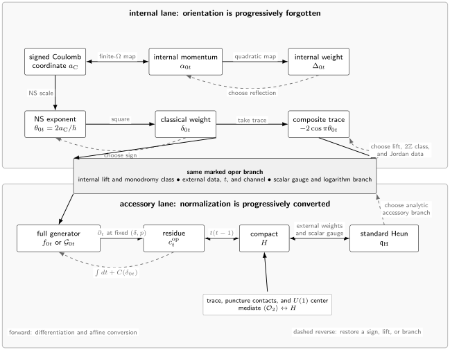
The internal and accessory lanes meet through a chosen generating-function branch. Squaring a momentum, taking a monodromy trace, and solving the inverse accessory problem lose different data. A standard-Heun number therefore does not point directly to a signed Coulomb modulus.

A full block generates the moving-pole residue

Let the full four-point background block in the marked channel be

$$\mathcal V_{0t}(t;b) = t^{ \Delta_{0t}-\Delta_0-\Delta_t } \widehat{\mathcal V}_{0t}(t;b).$$

On a chosen logarithm branch, assume the derivative-compatible classical limit

$$b^2\Log\mathcal V_{0t} \longrightarrow f_{0t}, \qquad b^2\partial_t\Log\mathcal V_{0t} \longrightarrow \partial_t f_{0t}.$$

Write

$$\kappa_{\mathrm{OPE}} := \delta_{0t}-\delta_0-\delta_t, \qquad f_{0t} = \kappa_{\mathrm{OPE}}\Log t + \widehat f_{0t}.$$

The moving-pole residue is

$$c_t^{\mathrm{op}} = \partial_t f_{0t} = \frac{\kappa_{\mathrm{OPE}}}{t} + \partial_t\widehat f_{0t}.$$

All derivatives here hold the external weights, internal lift, and analytic branch fixed. At generic $\delta_{0t}\neq0$, the level-one coefficient audits the regular part:

$$\widehat f_{0t} = \frac{ (\delta_{0t}+\delta_t-\delta_0) (\delta_{0t}+\delta_1-\delta_\infty) }{ 2\delta_{0t} } t+O(t^2).$$

This holomorphic chiral-block gradient is distinct from the rigorous Polyakov relation for the real uniformizing Liouville action. The two use different actions and stress-tensor normalizations; their signs and factors of $2\pi$ must not be transferred by name alone.

The pole is essential. In the sewing annulus $|t|\ll|z|\ll1$, it combines the two local double poles into

$$T_{\mathrm{op}}(z;t) = \frac{\delta_{0t}}{z^2} + O\left(\frac{t}{z^3}\right) + O\left(\frac1z\right).$$

Deleting the OPE power from the block but keeping the full-block accessory convention would replace $\delta_{0t}$ by $\delta_0+\delta_t$ and select the wrong composite channel.

Gauge and CFT derivatives agree only after the normalization gate

On the centered-mass NS path, Page 2 gives

$$\widehat f_{0t} = \frac1\hbar \left( \mathcal W_{\mathrm{NS}}^{U(2),\mathrm{inst}} - \mathcal W_{\mathrm{NS}}^{\mathcal H} \right),$$

where the same logarithm branch and fixed data $(p_f,a_{\mathrm C},\hbar)$ are used on both sides. The Heisenberg contribution is not negligible:

$$\mathcal W_{\mathrm{NS}}^{\mathcal H} = \frac{2}{\hbar} \left( p_1+\frac\hbar2 \right) \left( \frac\hbar2-p_t \right) \Log(1-t).$$

Therefore the branchwise gauge generating function

$$\mathcal G_{0t}(t) := \kappa_{\mathrm{OPE}}\Log t + \frac1\hbar \left( \mathcal W_{\mathrm{NS}}^{U(2),\mathrm{inst}} - \mathcal W_{\mathrm{NS}}^{\mathcal H} \right)$$

satisfies

$$c_t^{\mathrm{op}} = \partial_t\mathcal G_{0t}$$

in the normalized regular AGT package. Page 4 reaches the same coefficient by inserting the NS factorization into its exact coefficientwise finite-Omega defect equation in the local chart $0<|t|<1<|z|$:

$$c_t^{\mathrm{op}} = \frac1\hbar \partial_t\widetilde{\mathcal W}$$

for that page’s specified defect prefactor. This second equality is model-specific; changing the prefactor conjugates the differential operator and shifts the derivative.

For example, rescaling the underlying block or partition function by a multiplicative normalization—equivalently, adding the following logarithmic term to its generating function—

$$\mathcal G \longmapsto \mathcal G +A\Log t +B\Log(1-t) +C(a_{\mathrm C})$$

changes

$$c_t^{\mathrm{op}} \longmapsto c_t^{\mathrm{op}} +\frac At -\frac{B}{1-t},$$

and therefore

$$H \longmapsto H+A(t-1)+Bt.$$

The term $C(a_{\mathrm C})$ is invisible to the $t$ derivative. It can still change the coordinate conjugate to $a_{\mathrm C}$.

One accessory has four coordinate representatives

Use the Page 5 oriented external exponents and define

$$\begin{gathered} \gamma_{\mathrm H}=1-\theta_0, \qquad \delta_{\mathrm H}=1-\theta_1, \qquad \epsilon_{\mathrm H}=1-\theta_t, \\ \Lambda_\delta = \delta_\infty-\delta_0-\delta_t-\delta_1. \end{gathered}$$

The four-pole oper is

$$\begin{aligned} T_{\mathrm{op}}(z;t) ={}& \frac{\delta_0}{z^2} + \frac{\delta_t}{(z-t)^2} + \frac{\delta_1}{(z-1)^2} \\ &+ \frac{\Lambda_\delta}{z(z-1)} + \frac{ t(t-1)c_t^{\mathrm{op}} }{ z(z-1)(z-t) }. \end{aligned}$$

Define the compact coefficient and the Liouville-gauge coefficient by

$$H := t(t-1)c_t^{\mathrm{op}}, \qquad \mathcal K_{\mathrm H} := t\Lambda_\delta-H.$$

The standard-Heun accessory is

$$\mathfrak q_{\mathrm H} = \mathcal K_{\mathrm H} + \frac{\gamma_{\mathrm H}}2 \left( t\delta_{\mathrm H} +\epsilon_{\mathrm H} \right).$$

Combining the steps,

$$\begin{aligned} \mathfrak q_{\mathrm H} ={}& t\Lambda_\delta -t(t-1)c_t^{\mathrm{op}} \\ &+ \frac{\gamma_{\mathrm H}}2 \left( t\delta_{\mathrm H} +\epsilon_{\mathrm H} \right). \end{aligned}$$

Every arrow is algebraically reversible away from $t=0,1$:

$$c_t^{\mathrm{op}} = \frac{ t\Lambda_\delta +\frac{\gamma_{\mathrm H}}2 \left( t\delta_{\mathrm H} +\epsilon_{\mathrm H} \right) -\mathfrak q_{\mathrm H} }{ t(t-1) }.$$

This inverse recovers the normal-form equation. It does not yet recover $a_{\mathrm C}$: that requires the composite monodromy of this equation or inversion of the selected classical-block branch.

The weak cusp exposes the internal weight

The small-$t$ channel makes the inverse transparent. From

$$c_t^{\mathrm{op}} = \frac{ \delta_{0t}-\delta_0-\delta_t }{t} +O(1),$$

one obtains

$$\begin{aligned} \delta_{0t} &= \delta_0+\delta_t + \lim_{t\to0} t\,c_t^{\mathrm{op}} \\ &= \delta_0+\delta_t - \lim_{t\to0}H. \end{aligned}$$

Thus

$$\begin{aligned} \theta_{0t} &= \pm\sqrt{1-4\delta_{0t}}, \\ a_{\mathrm C} &= \pm\hbar \sqrt{ \frac14- \delta_0- \delta_t+ \lim_{t\to0}H } \end{aligned}$$

after choosing the internal exponent lift and Weyl orientation.

The standard-Heun coordinate has a finite cusp limit:

$$\mathfrak q_{\mathrm H}(0) = \frac{ \left( 1-\theta_0-\theta_t \right)^2 -\theta_{0t}^2 }{4}.$$

Hence a direct inverse seed is

$$\theta_{0t}^2 = \left( 1-\theta_0-\theta_t \right)^2 -4\mathfrak q_{\mathrm H}(0).$$

The geometry degenerates at $t=0$, so this is a limit in a marked sewing chart, not a four-puncture equation evaluated literally at the cusp.

At finite $t$, write the selected accessory branch schematically as

$$\mathfrak q_{\mathrm H} = \mathcal Q_{\mathrm H} \left( \delta_{0t},t;\boldsymbol\delta,\text{branch} \right).$$

The implicit-function inverse exists locally when $\partial_{\delta_{0t}}\mathcal Q_{\mathrm H}\neq0$. It can ramify, encounter a Kac pole, or continue to another analytic branch. A direct monodromy computation provides an independent inverse.

A rational round trip fixes every sign and scale

Take

$$\epsilon_1=\hbar=\frac52, \qquad \epsilon_2=\frac25, \qquad \varepsilon_\star=1, \qquad b=\frac25.$$

Choose $a_{\mathrm C}=3/4$. Then

$$Q_{\mathrm L}=\frac{29}{10}, \qquad \alpha_{0t}=\frac{11}{5}, \qquad \theta_{0t}=\frac35,$$

and

$$\Delta_{0t}=\frac{77}{50}, \qquad b^2\Delta_{0t}=\frac{154}{625}, \qquad \delta_{0t}=\frac4{25}.$$

The finite-Omega identity checks because

$$\frac{ (1+b^2)^2-\theta_{0t}^2 }{4} = \frac{154}{625}.$$

The lifted composite trace is

$$\operatorname{tr}M_{0t} = -2\cos\left(\frac{3\pi}{5}\right) = \frac{\sqrt5-1}{2}.$$

Now choose

$$\theta_0=\theta_t=\frac13, \qquad \theta_1=\theta_\infty=\frac15.$$

The cusp accessory is

$$\mathfrak q_{\mathrm H}(0) = -\frac{14}{225}.$$

Running the inverse gives

$$\theta_{0t}^2 = \frac19 -4\left(-\frac{14}{225}\right) = \frac9{25},$$

so $a_{\mathrm C}=\pm3/4$. The accessory cannot choose the Weyl sign; the original internal representative selects $+3/4$. The corresponding residue begins

$$c_t^{\mathrm{op}} = -\frac{64}{225t} +\frac2{25} +O(t),$$

and the scalar-gauge conversion gives the independent check

$$\mathfrak q_{\mathrm H}(t) = -\frac{14}{225} +\frac{14}{75}t +O(t^2).$$

Three derivatives move in three different directions

Let a normalized NS functional be fixed in one electric frame, mass scheme, and logarithm branch:

Derivative	Natural output	What must be fixed
$\partial_{a_{\mathrm C}}\mathcal W_{\mathrm{NS}}$	Coordinate conjugate to $a_{\mathrm C}$, often a quantum B-period	SW/WKB cycles, period factors, and electric frame
$t\partial_t\mathscr F_{\mathrm{NS}}$	Matone or quadratic chiral coordinate after calibration	Trace, coupling coordinate, contacts, and Abelian scheme
$\partial_t\mathcal G_{0t}$	Moving-pole oper residue	Full-block OPE power, defect or block prefactor, and scalar gauge

Even when $t=q_{\mathrm{UV}}$, these are not identities of notation. A model-specific Ward identity can relate the second and third rows, but it also supplies the mass contacts and trace factors. The first row belongs to the cycle dictionary of Page 7.

The chiral observable reaches H through contacts

The Page 4 defect supplies one such Ward identity. To compare its two coupling-derivative lanes, define

$$\widetilde{\mathscr F}_{\mathrm{NS}} := \hbar\widetilde{\mathcal W}, \qquad u_{\mathrm M}^{\mathrm{norm}} := -t\partial_t \widetilde{\mathscr F}_{\mathrm{NS}}.$$

The proved residue formula then implies

$$\begin{aligned} c_t^{\mathrm{op}} &= -\frac{ u_{\mathrm M}^{\mathrm{norm}} }{ \hbar^2t }, \\ H &= \frac{1-t}{\hbar^2} u_{\mathrm M}^{\mathrm{norm}}. \end{aligned}$$

This compact identity already contains a sign, a factor $1-t$, and two powers of $\hbar$. It is calibrated to the same defect prefactor as $c_t^{\mathrm{op}}=\hbar^{-1}\partial_t\widetilde{\mathcal W}$; it is not a convention-free definition of a Matone coordinate.

The source-normalized quadratic observable makes the missing affine terms explicit. Return to the uppercase Page 4 arrays and retain their $U(2)$ centers:

$$\bar A_i := \frac{A_{i,1}+A_{i,2}}2, \qquad \bar A_2 := \frac{A_{2,1}+A_{2,2}}2, \qquad i\in\{0,3\}.$$

and let $\mathcal O_2=\operatorname{Tr}\phi_2^2$ at the internal node. In this model,

$$\begin{aligned} H ={}& (1-t) \left[ \frac{1}{2\hbar^2} \lim_{\epsilon_2\to0} \langle\mathcal O_2\rangle -\frac14+\delta_t+\delta_0 \right] \\ &+ \frac{ 2(\bar A_0-\bar A_2) (\bar A_2-\bar A_3+\hbar) }{\hbar^2} t. \end{aligned}$$

Equivalently, the derivative-generated coordinate is

$$\begin{aligned} u_{\mathrm M}^{\mathrm{norm}} ={}& \frac12 \lim_{\epsilon_2\to0} \langle\mathcal O_2\rangle + \hbar^2 \left( -\frac14+\delta_t+\delta_0 \right) \\ &+ \frac{ 2(\bar A_0-\bar A_2) (\bar A_2-\bar A_3+\hbar) }{ 1-t } t. \end{aligned}$$

Solving for the observable gives the reverse map

$$\begin{aligned} \lim_{\epsilon_2\to0} \langle\mathcal O_2\rangle = 2\hbar^2 \Bigg[ &\frac{H}{1-t} +\frac14-\delta_t-\delta_0 \\ &- \frac{ 2t(\bar A_0-\bar A_2) (\bar A_2-\bar A_3+\hbar) }{ \hbar^2(1-t) } \Bigg]. \end{aligned}$$

The inverse is regular for $t\neq1$ once the trace convention, puncture weights, and centers are fixed. A local scheme change $\widetilde{\mathscr F}_{\mathrm{NS}}\mapsto \widetilde{\mathscr F}_{\mathrm{NS}}+C(t)$ shifts

$$u_{\mathrm M}^{\mathrm{norm}} \mapsto u_{\mathrm M}^{\mathrm{norm}}-tC'(t), \qquad c_t^{\mathrm{op}} \mapsto c_t^{\mathrm{op}}+\frac{C'(t)}{\hbar^2}.$$

Thus the relation survives a scheme change only after its contact terms are transformed with it.

At generic $a_{\mathrm C}$, the accessory is off shell: it is a holomorphic coordinate on a branch of the oper variety. A Bethe-vacuum condition may discretize $a_{\mathrm C}$, and a boundary problem may then select some of those values. Neither operation is part of the internal-to-accessory map itself.

Exceptional loci belong to different gates

Locus	Symptom	Consequence for the passport
Weyl fixed point $a_{\mathrm C}=0$	$\theta_{0t}=0$	The signed inverse branches meet
Internal Kac divisor	$2a_{\mathrm C}=-(r\epsilon_2+s\epsilon_1)$ up to reflection, $r,s\in\mathbb Z_{>0}$	Generic inverse-Gram or instanton chart develops a pole; a compatible quotient or limiting chart is needed
Composite trace resonance	$\theta_{0t}\in\mathbb Z$	The trace cannot decide Jordan data; use a Levelt or limiting prescription
Cusp degeneration	$t\in\{0,1,\infty\}$	The algebraic conversion through $t(t-1)$ degenerates; use the appropriate channel limit
Ramified accessory inverse	$\partial_{\delta_{0t}}\mathcal Q_{\mathrm H}=0$	Several internal branches meet over one accessory value
Endpoint Heun normalization	$\gamma_{\mathrm H}\in\mathbb Z_{\leq0}$	The direct exponent-zero HeunG germ can be obstructed or nonunique

Indeed, the finite-Omega Kac condition gives

$$2a_{\mathrm C} = -(r\epsilon_2+s\epsilon_1) \quad\Longrightarrow\quad \theta_{0t}^{[1]} = -(rb^2+s).$$

Here $r,s\in\mathbb Z_{>0}$. The divisor is generally not a composite-trace resonance at finite $b$, though for fixed $(r,s)$ it approaches the integer $-s$ on this NS path.

These tests answer different questions. In particular, an internal Kac pole is not an endpoint Frobenius resonance, and neither one is by itself a spectral condition.

A reversible internal passport

Internal lane

Map	Forward	Reverse	Gate
$a_{\mathrm C}\leftrightarrow\alpha_{0t}$	$\alpha_{0t}=Q_{\mathrm L}/2+a_{\mathrm C}/\varepsilon_\star$	$a_{\mathrm C}=\varepsilon_\star(\alpha_{0t}-Q_{\mathrm L}/2)$	Square-root branch and Weyl orientation; AGT §3.2
$a_{\mathrm C}\leftrightarrow\theta_{0t}$	$\theta_{0t}=2a_{\mathrm C}/\hbar$	$a_{\mathrm C}=\hbar\theta_{0t}/2$	Ordered Omega plane and centered NS path
$\theta_{0t}\leftrightarrow\delta_{0t}$	$\delta_{0t}=(1-\theta_{0t}^2)/4$	$\theta_{0t}=\pm\sqrt{1-4\delta_{0t}}$	Weyl sign lost
$\theta_{0t}\leftrightarrow\operatorname{tr}M_{0t}$	$\operatorname{tr}M_{0t}=-2\cos(\pi\theta_{0t})$	Inverse cosine with sign and $2\mathbb Z$ branch	Marked loop, determinant-one lift, and Jordan data; Litvinov et al. Eq. (2.15)

Accessory lane

Map	Forward	Reverse	Gate
$f_{0t}\leftrightarrow c_t^{\mathrm{op}}$	$c_t^{\mathrm{op}}=\partial_t f_{0t}$	$f_{0t}=\int c_t^{\mathrm{op}}\,dt+C(\delta_{0t})$	Classical limit, full-block normalization, and branch
$\mathcal G_{0t}\leftrightarrow c_t^{\mathrm{op}}$	$c_t^{\mathrm{op}}=\partial_t\mathcal G_{0t}$	Integrate at fixed internal data	Centered masses, Heisenberg subtraction, OPE power, and prefactor
$c_t^{\mathrm{op}}\leftrightarrow H$	$H=t(t-1)c_t^{\mathrm{op}}$	$c_t^{\mathrm{op}}=H/[t(t-1)]$	$t\neq0,1$
$H\leftrightarrow\mathcal K_{\mathrm H}$	$\mathcal K_{\mathrm H}=t\Lambda_\delta-H$	$H=t\Lambda_\delta-\mathcal K_{\mathrm H}$	External weights fixed
$\mathcal K_{\mathrm H}\leftrightarrow\mathfrak q_{\mathrm H}$	Add or subtract $\gamma_{\mathrm H}(t\delta_{\mathrm H}+\epsilon_{\mathrm H})/2$	Same affine step reversed	Oriented endpoint exponents and scalar gauge; DLMF §31.2
$\langle\mathcal O_2\rangle\leftrightarrow H$	Use the displayed trace-and-contact map	Solve the same affine relation for $\langle\mathcal O_2\rangle$	Trace, puncture contacts, $U(1)$ centers, and $t\neq1$; Jeong–Nekrasov Eq. (3.23)

No row identifies $a_{\mathrm C}$ with $H$, $\mathfrak q_{\mathrm H}$, or $u_2$. The relation among them is a normalized, branchwise map, not a change of symbols.

Reverse-engineering Coulomb data from a Heun equation

Given a standard Heun equation rather than gauge data, the inverse workflow is:

1. Mark the punctures and scalar gauge, then read $(t,\alpha_{\mathrm H},\beta_{\mathrm H}, \gamma_{\mathrm H},\delta_{\mathrm H}, \epsilon_{\mathrm H},\mathfrak q_{\mathrm H})$, together with the Fuchs relation.
2. Reconstruct the oriented exponent representatives and external weights, then use the affine Heun formula to obtain $c_t^{\mathrm{op}}$.
3. Continue normalized local bases along the declared loops and compute the composite matrix $M_0M_t$.
4. Lift its trace to an exponent representative $\theta_{0t}$, retaining the exponent lattice and any resonant Jordan data.
5. Set $a_{\mathrm C}=\hbar\theta_{0t}/2$ only after choosing the Weyl orientation. Near $t=0$, audit that choice against the cusp residue or $\mathfrak q_{\mathrm H}(0)$.

Integrating $c_t^{\mathrm{op}}$ instead reconstructs a generating function only up to $C(\delta_{0t})$. That missing term is invisible to the accessory but can change the conjugate twist or B-period.

Where the internal passport stops

The completed passport fixes a scalar differential equation on a chosen oper branch. It does not by itself provide:

• a normalized connection matrix between endpoint bases;
• the twist coordinate conjugate to $\theta_{0t}$;
• a choice of SW, monodromy, or WKB cycle;
• a Bethe vacuum or other on-shell constraint;
• a self-adjoint, resonant, or quasinormal boundary condition;
• a nonperturbative completion in $\hbar$.

Page 7 aligns the three cycle languages. Page 8 then adds the remaining normalization and spectral gates in a complete connection-formula example.

Confluence changes the passport

The regular table is not carried unchanged through a decoupling limit. When punctures collide while masses and $t$ scale, the finite quantity may be a scale derivative or an irregular Hamiltonian rather than $\partial_t f$, and ordinary composite monodromy is replaced in part by formal monodromy and Stokes data. The factor $t(t-1)$ can simultaneously vanish while the rescaled irregular accessory stays finite. Use the confluent dictionary before taking such a limit.

Common pitfalls

Calling the internal momentum a local exponent. It controls the composite $0t$ monodromy, not a fifth endpoint. Its weight is absent from the four local double poles.

Calling the Coulomb coordinate an accessory. Fixing $a_{\mathrm C}$ selects an accessory only after the external data, coupling, channel, normalization, and analytic branch are fixed.

Differentiating the hatted block as if it were full. This drops $\kappa_{\mathrm{OPE}}/t$ and fails the sewing-annulus check.

Equating a raw localization derivative with Heun’s $\mathfrak q_{\mathrm H}$. The derivative first produces a normal-form residue after normalization; two further affine conversions remain.

Recovering a signed period from a trace. A trace loses the Weyl sign, exponent lattice, and resonant Jordan information.

Putting the accessory on shell automatically. Generic $a_{\mathrm C}$ produces a continuous oper family. Quantization needs an independent vacuum or boundary condition.

Exercises

1. Check the finite-Omega internal weight

Starting from $\alpha_{0t}=Q_{\mathrm L}/2+a_{\mathrm C}/\varepsilon_\star$, derive $\Delta_{0t}$ in dimensionful variables and then derive the finite-$b$ identity for $b^2\Delta_{0t}$.

Solution

Using $Q_{\mathrm L}=\epsilon_\Sigma/\varepsilon_\star$ and $\varepsilon_\star^2=\epsilon_1\epsilon_2$ gives

$$\Delta_{0t} = \frac{ \epsilon_\Sigma^2-4a_{\mathrm C}^2 }{ 4\epsilon_1\epsilon_2 }.$$

With $\theta_{0t}^{[1]}=2a_{\mathrm C}/\epsilon_1$ and $b^2=\epsilon_2/\epsilon_1$,

$$b^2\Delta_{0t} = \frac{ (1+b^2)^2- \left(\theta_{0t}^{[1]}\right)^2 }{4}.$$

2. Invert a composite trace

In the natural scalar lift, suppose $\operatorname{tr}M_{0t}=0$. List the possible internal exponent representatives and the additional datum needed to choose $a_{\mathrm C}$.

Solution

The equation $-2\cos(\pi\theta_{0t})=0$ gives

$$\theta_{0t} = \frac12+n, \qquad n\in\mathbb Z.$$

Equivalently one may write the inverse with the explicit $\pm$ and $2\mathbb Z$ branches. A logarithm branch chooses an exponent representative; the Coulomb Weyl orientation chooses its sign before $a_{\mathrm C}=\hbar\theta_{0t}/2$ is assigned.

3. Conjugate the generating function

Let $\mathcal G'=\mathcal G+A\Log t+B\Log(1-t)+C(a_{\mathrm C})$. Find the new moving-pole residue.

Solution

At fixed $a_{\mathrm C}$,

$$\partial_t\mathcal G' = c_t^{\mathrm{op}} +\frac At -\frac{B}{1-t}.$$

The $t$-independent function $C$ is invisible to the accessory derivative, although it shifts the conjugate Coulomb coordinate under an $a_{\mathrm C}$ derivative.

4. Recover the internal weight at the cusp

Show that the coefficient of $1/t$ in $c_t^{\mathrm{op}}$ determines $\delta_{0t}$. Then derive the direct formula in terms of $\mathfrak q_{\mathrm H}(0)$.

Solution

From full-block sewing,

$$\lim_{t\to0}t\,c_t^{\mathrm{op}} = \delta_{0t}-\delta_0-\delta_t.$$

Therefore

$$\delta_{0t} = \delta_0+\delta_t + \lim_{t\to0}t\,c_t^{\mathrm{op}}.$$

Using the scalar-gauge conversion at the cusp gives

$$\theta_{0t}^2 = \left( 1-\theta_0-\theta_t \right)^2 -4\mathfrak q_{\mathrm H}(0).$$

5. Reproduce the rational inverse

Use $\theta_0=\theta_t=1/3$ and $\mathfrak q_{\mathrm H}(0)=-14/225$ to recover $\theta_{0t}$ and $a_{\mathrm C}$ when $\hbar=5/2$.

Solution

The cusp formula gives

$$\theta_{0t}^2 = \frac19+\frac{56}{225} = \frac9{25}.$$

Thus $\theta_{0t}=\pm3/5$ and

$$a_{\mathrm C} = \frac{\hbar\theta_{0t}}2 = \pm\frac34.$$

The accessory fixes the Weyl orbit. The declared internal representative is needed to select one sign.

6. Separate the derivative lanes

Explain why adding a $t$-independent one-loop term can leave the accessory unchanged but alter a B-period relation.

Solution

If $C=C(a_{\mathrm C})$ is independent of $t$, then $\partial_tC=0$, so $c_t^{\mathrm{op}}$ is unchanged. In general $\partial_{a_{\mathrm C}}C\neq0$, so the coordinate conjugate to $a_{\mathrm C}$ and any B-period comparison shift. “Invisible to one derivative” does not mean physically irrelevant.

7. Diagnose a ramified inverse

Why does the cusp inverse fail to distinguish branches at $\theta_{0t}=0$?

Solution

At the cusp,

$$\partial_{\theta_{0t}} \mathfrak q_{\mathrm H}(0) = -\frac{\theta_{0t}}2.$$

The derivative vanishes at $\theta_{0t}=0$, where the two Weyl-related square-root branches meet. One should use the invariant coordinate $\delta_{0t}$ there and impose any required resonant or limiting data separately.

8. Audit the Matone contacts at the cusp

In the rational example, take the zero-coupling traceless-center value $\frac12\langle\mathcal O_2\rangle=a_{\mathrm C}^2$. Show that the contact-corrected $u_{\mathrm M}^{\mathrm{norm}}(0)$ reproduces the $1/t$ coefficient of $c_t^{\mathrm{op}}$.

Solution

Here

$$\delta_0=\delta_t=\frac29, \qquad \frac12\langle\mathcal O_2\rangle = a_{\mathrm C}^2 = \frac9{16}.$$

The puncture contact is

$$\hbar^2 \left( -\frac14+\delta_t+\delta_0 \right) = \frac{25}{4}\frac7{36} = \frac{175}{144}.$$

Consequently,

$$u_{\mathrm M}^{\mathrm{norm}}(0) = \frac9{16}+\frac{175}{144} = \frac{16}{9}.$$

Because $c_t^{\mathrm{op}}=-u_{\mathrm M}^{\mathrm{norm}}/(\hbar^2t)$,

$$c_t^{\mathrm{op}} = -\frac{16}{9}\frac4{25t} +O(1) = -\frac{64}{225t} +O(1),$$

which is the OPE residue found in the round trip.

References

• L. F. Alday, D. Gaiotto, and Y. Tachikawa, “Liouville Correlation Functions from Four-Dimensional Gauge Theories”, Letters in Mathematical Physics 91 (2010), 167–197. Section 3.2, especially equations (3.5)–(3.13), fixes the internal momentum, Coulomb coordinate, four-point block, and Heisenberg factor. The paper states the correspondence conjecturally and tests its formal series; this page adopts that normalized correspondence coefficientwise.
• A. Litvinov, S. Lukyanov, N. Nekrasov, and A. Zamolodchikov, “Classical Conformal Blocks and Painlevé VI”, Journal of High Energy Physics 07 (2014) 144. Equations (1.8), (2.7)–(2.10), and (2.13)–(2.19) give the full classical block, four-pole oper, accessory gradient, composite trace, and conjugate-twist caveat.
• S. Jeong and N. Nekrasov, “Opers, Surface Defects, and Yang–Yang Functional”, Advances in Theoretical and Mathematical Physics 24 (2020), 1789–1916. Equations (3.14)–(3.23), (6.9)–(6.12), and (6.18)–(6.26) give the source arrays, finite-Omega defect identity, NS accessory and contact map, composite trace, one-loop caveat, and all-orders formal four-puncture $SL(2)$ generating-function relation.
• F. Ferrari and M. Piątek, “Liouville Theory, N=2 Gauge Theories and Accessory Parameters”, Journal of High Energy Physics 05 (2012) 025. Equations (2.28), (2.40), and (3.22)–(3.24) relate the four-point classical-block derivative to the NS instanton saddle and display the Abelian logarithmic shift.
• L. A. Takhtajan and P. G. Zograf, “Hyperbolic 2-Spheres with Conical Singularities, Accessory Parameters and Kähler Metrics on $\mathcal M_{0,n}$”, Transactions of the American Mathematical Society 355 (2003), 1857–1867. The published Theorem 1 gives the Polyakov relation for the real uniformizing action under its geometric hypotheses; its normalization is deliberately kept separate from the holomorphic block gradient used here.
• J. Teschner, “Classical Conformal Blocks and Isomonodromic Deformations”, 2017. Develops classical blocks as local generating functions between oper and monodromy Darboux coordinates and makes the branch dependence explicit.
• M. Piątek and A. R. Pietrykowski, “Solving Heun’s Equation Using Conformal Blocks”, Nuclear Physics B 938 (2019), 543–570. Provides a normalization-aware classical-block derivation of Heun solutions and accessory data.
• NIST Digital Library of Mathematical Functions, §31.2 and §31.3(i). These sections define the standard Heun accessory, exponent ledger, normal-form conversion, and normalized local solution together with its exceptional parameters.