Pure Quartic Oscillator: From TBA to Exact Levels

The pure quartic oscillator is where every gate needed for one complete TBA-to-spectrum calculation can be closed without changing models. Starting from one two-function TBA, we will reconstruct a median-resummed real action and a complex-instanton action, impose the exact real-line quantization condition, and obtain the first six eigenvalues of $-\partial_q^2+q^4$. A parity-resolved matrix calculation then reproduces the same numbers independently.

The example is deliberately normalization-complete. The TBA unknowns first serve as WKB-period coordinates. They become spectral data only after the $L^2(\mathbb R)$ boundary condition and the quartic exact quantization condition have been supplied. A second, ODE/IM identification maps a different output of the same TBA solution to a spectral determinant. These two output maps agree here; neither is a definition valid for an arbitrary TBA.

Status ledger

Statement	Status in this example
Scaling between fixed energy and the ordinary quartic spectrum	Exact change of variables
Maximal-chamber charge set and period reconstruction	Published model-specific exact-WKB construction
Six charges reducing to two orbit functions	Exact at the pure-quartic symmetry point after the stated wall-crossing route
Folded TBA matching the $A_3$ ODE/IM equation	Equation-level identity with matched rapidity, masses, kernels, logarithms, and asymptotics
Real-axis quantization condition	Published pure-quartic exact-WKB condition with median/lateral prescriptions fixed
TBA solution selected below	Numerical fixed point with asymptotic and refinement audits; no global complex uniqueness theorem is claimed
Determinant functional relation	Exact ODE identity in the stated determinant normalization
Six displayed levels	Reproducible double-precision evidence, independently checked; not interval-certified values
NS interpretation	Not used and not inferred

The quartic passport turns inverse ℏ into energy

Fix the energy of the semiclassical problem to one:

$$\left[ -\hbar^2\frac{\dd^2}{\dd q^2} +q^4-1 \right]\psi(q)=0, \qquad \psi\in L^2(\mathbb R), \qquad \hbar>0.$$

Put $q=\hbar^{1/3}z$. Dividing the transformed equation by $\hbar^{4/3}$ gives

$$\left[ -\frac{\dd^2}{\dd z^2}+z^4 \right]\psi(z) = \hbar^{-4/3}\psi(z).$$

It is therefore useful to define

$$X=\hbar^{-1}, \qquad \theta=\log X=-\log\hbar.$$

If $E_n$ denotes the $n$th eigenvalue of

$$H_4=-\frac{\dd^2}{\dd z^2}+z^4 \quad\text{on }L^2(\mathbb R),$$

then the fixed-energy roots and ordinary energies obey

$$E_n=X_n^{4/3}, \qquad X_n=\ee^{\theta_n}, \qquad \hbar_n=X_n^{-1}.$$

This exponent is easy to lose if one imports a table computed with $-(\hbar^2/2)\partial_q^2+q^4/2$. That Hamiltonian is one half of the operator above. Its fixed energy $1/2$, not $1$, represents the same problem.

The complete passport is short enough to keep visible throughout the calculation.

Entry	Convention used below
Scaled ODE	$[-\hbar^2\partial_q^2+q^4-1]\psi=0$
Boundary domain	Real line, decay at both ends
Turning points	$1,\ii,-1,-\ii$ in the $q$-plane
Real cycle	$\gamma_{123}$, oriented so its classical action is positive
Complex cycle	$\gamma_2$, with $\ii\Pi_{\gamma_2}/\hbar>0$ on the chosen ray
Chamber	Final maximal pure-quartic chamber, reached before symmetry reduction
Rapidity	$\theta=-\log\hbar$
TBA logarithm	$L_a=\log(1+\ee^{-\varepsilon_a})$
Real action	Median sum on the positive-$\hbar$ Stokes direction
Complex action	Declared Borel sum transported with the same chamber passport
State labels	Even $n$: even/Neumann; odd $n$: odd/Dirichlet
Observable	$E_n=\exp(4\theta_n/3)$

For readers following the ODE/IM normalization of Chapter 12, the same point has

$$\begin{gathered} M=2, \qquad l=0, \qquad \beta^2=\frac13, \qquad p=\frac1{12}, \\ q_{\mathrm{rot}}=\ee^{\pi\ii/3}, \qquad s=v_2E, \qquad v_2= 6^{-4/3}\Gamma\!\left(\frac23\right)^{-2}. \end{gathered}$$

Numerically, $v_2\approx0.0500209592727608$. The symbol $q_{\mathrm{rot}}$ is a rotation parameter and is unrelated to the coordinate $q$ in the fixed-energy equation.

Six chamber charges collapse to two orbit masses

The minimal quartic chamber starts with three adjacent cycles $\gamma_1,\gamma_2,\gamma_3$. Continuing to the maximal chamber activates

$$\gamma_{12}=\gamma_1+\gamma_2, \qquad \gamma_{23}=\gamma_2+\gamma_3, \qquad \gamma_{123}=\gamma_1+\gamma_2+\gamma_3.$$

Thus the generic maximal-chamber problem has six coordinates. Reflection first identifies $1$ with $3$ and $12$ with $23$. At the pure-quartic point the enhanced $\mathbb Z_4$ symmetry further identifies the orbit of $1$ with that of $12$, and the orbit of $2$ with that of $123$. Only then do two independent functions remain. This is the route

$$3\text{ minimal charges} \longrightarrow 6\text{ maximal charges} \longrightarrow 2\text{ symmetry orbits}.$$

It must not be replaced by deleting four functions from a generic six-function system. Page 5 showed why the intervening composite charges are necessary during wall crossing.

The larger drive mass is shared by the complex cycle $\gamma_2$ and the real cycle $\gamma_{123}$. In the orientations fixed by the passport,

$$\begin{aligned} m_2 &:= |m_{\gamma_2}| =|m_{\gamma_{123}}| =\Pi_{\gamma_{123}}^{(0)} \\ &= 4\int_0^1\sqrt{1-q^4}\,\dd q \\ &= B\!\left(\frac14,\frac32\right) = \frac{\sqrt\pi\,\Gamma(\frac14)} {2\Gamma(\frac74)} = \frac83K(\ii). \end{aligned}$$

The corresponding leading complex action is $\Pi_{\gamma_2}^{(0)}=-\ii m_2$. Thus $\ii\Pi_{\gamma_2}^{(0)}/\hbar$ and $\Pi_{\gamma_{123}}^{(0)}/\hbar$ are both positive in the two real quantities reconstructed below.

Here $K(\ii)$ denotes the complete elliptic integral with modulus $\ii$; a library whose argument is the elliptic parameter receives $m=-1$. Rotation symmetry gives the other mass:

$$\begin{aligned} m_1&=\frac{m_2}{\sqrt2} =\frac{4\sqrt2}{3}K(\ii), \\ m_1&\approx2.47209956973516, \qquad m_2\approx3.49607673905616. \end{aligned}$$

The ratio $m_2/m_1=\sqrt2$ is both a WKB period check and the Perron–Frobenius mass ratio of the folded $A_3$ system. A common rapidity translation can change their overall scale, but not this ratio.

The folded system is the whole nonlinear solve

For

$$(K*f)(\theta) = \int_{\mathbb R} K(\theta-t)f(t)\,\dd t, \qquad L_a(\theta)=\log(1+\ee^{-\varepsilon_a(\theta)}),$$

the two orbit pseudoenergies satisfy

$$\begin{aligned} \varepsilon_1(\theta) &= m_1\ee^\theta +(\kappa_0*L_1)(\theta) +(\kappa_1*L_2)(\theta), \\ \varepsilon_2(\theta) &= m_2\ee^\theta +2(\kappa_1*L_1)(\theta) +(\kappa_0*L_2)(\theta), \end{aligned}$$

with

$$\kappa_0(u)=\frac{1}{\pi\cosh u}, \qquad \kappa_1(u)= \frac{\sqrt2}{\pi} \frac{\cosh u}{\cosh(2u)}.$$

The asymmetric factor of two remembers that the central $A_3$ node has two reflected neighbors. Both kernels have integral one. Consequently a constant left plateau must obey

$$\varepsilon_1^-=L_1^-+L_2^-, \qquad \varepsilon_2^-=2L_1^-+L_2^-.$$

The solution is

$$(\varepsilon_1^-,\varepsilon_2^-) =(\log2,\log3),$$

because $L_1^-=\log(3/2)$ and $L_2^-=\log(4/3)$. This one-line audit detects a missing orbit multiplicity, a reciprocal-$Y$ convention, or an incorrect kernel measure before any spectrum is computed.

Which TBA is being solved?

This positive-kernel folded equation is simultaneously the final pure-quartic exact-WKB reduction and the reflection-folded $A_3$ ODE/IM equation after the Page 4 dictionary is applied. It is not the raw minimal-chamber negative-convolution equation. Dorey and Tateo also use a $Y=\ee^{+\varepsilon}$ convention in part of the original discussion; copying a displayed formula without transporting that choice reverses the nonlinear asymptotics.

A real-line solver integrates both tails analytically

The companion calculation uses an odd uniform grid on $[-T,T]$ and zero-padded Toeplitz FFTs. It never treats the convolution as periodic. The nonzero left limits of $L_1$ and $L_2$ are integrated analytically against both kernels, while the right tails vanish superexponentially because of the drives. Plain Picard iteration then converges on the real branch selected by the plateaux and right asymptotics.

The complete NumPy implementation is pure-quartic-tba-spectrum.py. Run its default refinement audit with

python3 public/code/advanced-ode/pure-quartic-tba-spectrum.py

and add the high-resolution grid with

python3 public/code/advanced-ode/pure-quartic-tba-spectrum.py \
  --high --figure-data

The high run uses $T=30$ and $N=65537$. Its fixed-point residual is $5.7\times10^{-14}$. On a separate 65-point audit grid, each zero-padded FFT convolution agrees with direct dense Nyström multiplication to $2.3\times10^{-16}$ or better. The code also checks the mass ratio, both plateau equations, every bracketed root, and the independent Rayleigh–Ritz refinement.

These tests play different roles. The nonlinear residual tests the discrete fixed point; the dense multiplication tests the FFT embedding; the cutoff and mesh comparison probes continuum discretization; and the direct Hamiltonian tests the final observable. None can substitute for the others.

Median and complex periods require different formulas

Define the positive complex-cycle action

$$\mathcal B(\theta) = \frac{\ii}{\hbar} s\!\left(\Pi_{\gamma_2}\right)(\hbar) = \varepsilon_2(\theta)>0,$$

and the median real-cycle action

$$\mathcal A(\theta) = \frac{1}{\hbar} s_{\mathrm{med}}\!\left( \Pi_{\gamma_{123}} \right)(\hbar).$$

Here $\varepsilon_a$ denotes the real-axis folded function $\widetilde\varepsilon_a$ of Ito–Mariño–Shu Eq. (5.29), with the cycle orientation fixed in the passport above. Transporting their period dictionary in Eq. (3.6) through the maximal-chamber phases of Eq. (5.22) and the pure-quartic symmetry of Eq. (5.28) gives $\mathcal B=\varepsilon_2$; it is not an unshifted minimal-chamber formula copied verbatim. The real cycle lies on a Stokes direction and is not given by simply reading off $\varepsilon_1$.

Specializing the median reconstruction in Ito–Mariño–Shu Eq. (5.24) to $\alpha=\pi/4$ and using $\widetilde L_1=\widetilde L_{12}$ from Eq. (5.28) yields

$$\begin{aligned} \mathcal A(\theta) ={}&m_2\ee^\theta -\frac{2\sqrt2}{\pi} \int_{\mathbb R} \frac{\sinh(\theta-t)} {\cosh\!\left(2(\theta-t)\right)} L_1(t)\,\dd t \\ &- \frac1\pi\operatorname{PV} \int_{\mathbb R} \frac{L_2(t)}{\sinh(\theta-t)}\,\dd t. \end{aligned}$$

The last kernel has a pole at $t=\theta$. Numerically, use the exact singularity subtraction

$$\operatorname{PV} \int_{\mathbb R} \frac{L_2(t)}{\sinh(\theta-t)}\,\dd t = \int_{\mathbb R} \frac{L_2(t)-L_2(\theta)} {\sinh(\theta-t)}\,\dd t.$$

The diagonal limit of the new integrand is $-L_2'(\theta)$. The code interpolates both $L_2(\theta)$ and this derivative locally, includes the analytic plateau tails of the subtracted integral, and applies composite Simpson quadrature only to the smooth remainder. Introducing an arbitrary hole $|t-\theta|>\delta$ would add an uncontrolled parameter precisely in the term that carries the median prescription.

The analytic-continuation firewall remains visible

The formulas above live on the real rapidity axis with declared summation banks. A determinant zero can also be described after the complex shift $\theta\mapsto\theta+3\pi\ii/4$, but that path crosses kernel singularities. Continue with the $Y$-system or the corresponding residue formula; do not insert the shifted argument into the first-strip convolution.

The exact condition separates even and odd levels

Ito–Mariño–Shu write the relevant condition as Eq. (5.25) in the above-barrier quartic chamber and explicitly extend the same TBA system and condition to $\kappa\leq0$ after Eq. (5.26). The equation below is its pure-quartic specialization at $\kappa=0$.

For level label $n=0,1,\ldots$, define

$$\mathcal J_n(\theta) = \mathcal A(\theta) -2(-1)^n \tan^{-1}\!\left( \ee^{-\mathcal B(\theta)/2} \right).$$

The real-line $L^2$ spectrum is selected by

$$\mathcal J_n(\theta_n) = 2\pi\left(n+\frac12\right).$$

Equivalently, the two curves drawn below are

$$\begin{aligned} \mathcal J_{\mathrm{even}} &= \mathcal A-2\tan^{-1}(\ee^{-\mathcal B/2}), \qquad n=0,2,4,\ldots, \\ \mathcal J_{\mathrm{odd}} &= \mathcal A+2\tan^{-1}(\ee^{-\mathcal B/2}), \qquad n=1,3,5,\ldots. \end{aligned}$$

Even $n$ gives an even full-line eigenfunction, equivalently a Neumann half-line problem at the origin. Odd $n$ gives an odd eigenfunction and a Dirichlet half-line problem. At large $n$, $\mathcal B$ grows and the arctangent is exponentially small, leaving the all-orders Bohr–Sommerfeld structure. For the ground state it changes the action by about $0.277$ and cannot be omitted.

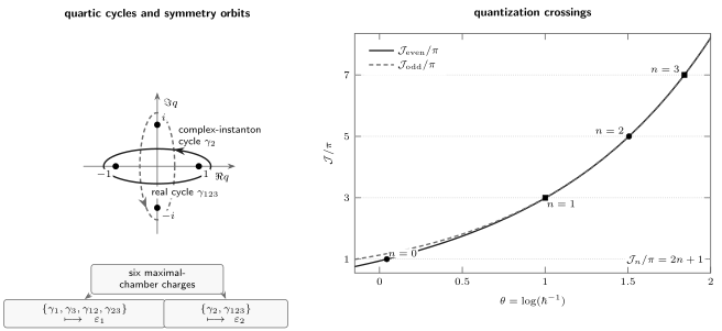
Left: the four turning points of $q^4=1$, the $q$-plane projections of the real and complex cycles entering the exact condition, and the six-charge-to-two-function orbit reduction. Right: the parity-sensitive functions $\mathcal J_{\mathrm{even}}/\pi$ and $\mathcal J_{\mathrm{odd}}/\pi$ cross the odd-integer quantization lines. Only the parity-compatible marked crossings are levels. The curves merge rapidly as the complex-cycle correction becomes exponentially small.

Bisection is used only after a sign-changing interval has been found. On the high grid, the resulting energies are:

$n$	parity	$X_n=\hbar_n^{-1}$	$E_n$ from TBA	Rayleigh–Ritz $E_n$	absolute discrepancy
0	even/N	1.0449382925090	1.060362090484179	1.060362090484184	$5.6\times10^{-15}$
1	odd/D	2.7215083408354	3.799673029801393	3.799673029801394	$4.4\times10^{-16}$
2	even/N	4.5119702604656	7.455697937986746	7.455697937986748	$1.8\times10^{-15}$
3	odd/D	6.3037285199589	11.644745511378165	11.644745511378158	$7.1\times10^{-15}$
4	even/N	8.0979852755214	16.261826018850229	16.261826018850250	$2.1\times10^{-14}$
5	odd/D	9.8932943734278	21.238372918235950	21.238372918235942	$7.1\times10^{-15}$

The many digits are printed to expose the independent comparison, not to claim a certified error bar. A more conservative portable report of the result is the first twelve significant digits of each energy. At fixed step $h=0.0018310546875$, changing $T=22.5$ to $T=30$ moves any displayed level by at most $2.5\times10^{-15}$. At fixed $T=30$, changing $N=32769$ to $N=65537$ moves any level by at most $4.8\times10^{-14}$.

Both numerical columns are computations made by the companion code. Rounded to the precision of Dorey–Tateo Table I, the TBA column also agrees with all six published pure-$q^4$ levels. That table is the literature determinant/TBA benchmark; the Rayleigh–Ritz column is the independent calculation performed here.

The period ledger shows directly how the nonperturbative term alternates:

$n$	$\mathcal B(\theta_n)$	$\mathcal A(\theta_n)$	$2(-1)^n\tan^{-1}(\ee^{-\mathcal B/2})$	EQC residual
0	3.938425611354309	3.418934503841784	$+0.277341850251995$	$-4.0\times10^{-15}$
1	9.627034960524387	9.408539817364582	$-0.016238143404796$	$0$
2	15.841285504565230	15.708689605564786	$+0.000726337615808$	$1.2\times10^{-14}$
3	22.086115145332105	21.991116579471846	$-0.000031995656710$	$3.6\times10^{-15}$

The sign of the correction in $\mathcal J_n$ matters: the table lists the quantity being subtracted from $\mathcal A$.

The determinant supplies a second spectral gate

Let $D_{\mathrm{DT}}$ be the full-line zeta determinant in the Dorey–Tateo normalization,

$$D_{\mathrm{DT}}(z) = 2\prod_{n=0}^{\infty} \left(1+\frac{z}{E_n}\right), \qquad D_{\mathrm{DT}}(0)=2.$$

The model-specific ODE/IM output map is

$$\begin{aligned} \ee^{\varepsilon_1(\theta)} &= D_{\mathrm{DT}}\!\left(\ee^{4\theta/3}\right) \\ &= 2Q_+\!\left( -v_2\ee^{4\theta/3},\frac1{12} \right) Q_-\!\left( -v_2\ee^{4\theta/3},\frac1{12} \right). \end{aligned}$$

Each normalized half-line determinant has $Q_\pm(0)=1$; the prefactor $2$ is therefore precisely the full-line zeta normalization $D_{\mathrm{DT}}(0)=2$. The physical roots occur at the negative determinant argument $z=-E_n$:

$$\begin{array}{lll} n=2k: &Q_-(v_2E_n,1/12)=0, &\text{even/Neumann}, \\ n=2k+1: &Q_+(v_2E_n,1/12)=0, &\text{odd/Dirichlet}. \end{array}$$

With $j=\ee^{2\pi\ii/3}$, the determinant also obeys the exact quartic functional relation

$$\begin{aligned} D_{\mathrm{DT}}(j^{-1}z) D_{\mathrm{DT}}(z) D_{\mathrm{DT}}(jz) ={}&D_{\mathrm{DT}}(j^{-1}z) \\ &+D_{\mathrm{DT}}(z) +D_{\mathrm{DT}}(jz)+2. \end{aligned}$$

At $z=0$ it reads $8=6+2$, a sharp normalization audit. The determinant identity does not say that $\varepsilon_2$ is a determinant or that $\mathcal A$ can be discarded. Rather, the common TBA solution has a period reconstruction used by the real exact-WKB condition and a determinant reconstruction used by ODE/IM. Their agreement after both boundary passports are imposed is the substantive check.

The determinant lane here is an exact structural and literature audit: the companion code does not separately continue the $Y$-system and evaluate $D_{\mathrm{DT}}(-E_n)$ at all six roots. The independent numerical audit on this page is the Rayleigh–Ritz calculation below.

Direct diagonalization closes the numerical audit

For an independent calculation, expand $H_4=p^2+q^4$ in harmonic-oscillator states of adjustable frequency $\omega$. Parity makes the matrix block diagonal. Its nonzero upper bands are

$$\begin{aligned} (H_4)_{n,n} ={}& \frac{\omega}{2}(2n+1) +\frac{3(2n^2+2n+1)}{4\omega^2}, \\ (H_4)_{n,n+2} ={}& \sqrt{(n+1)(n+2)} \left[ -\frac{\omega}{2} +\frac{2n+3}{2\omega^2} \right], \\ (H_4)_{n,n+4} ={}& \frac{ \sqrt{(n+1)(n+2)(n+3)(n+4)} }{4\omega^2}. \end{aligned}$$

All other entries follow by symmetry or vanish. The companion script diagonalizes the even and odd blocks separately, interlaces their lowest eigenvalues, and varies the basis dimension and $\omega$. Around a 120-state basis and $\omega=6$, the largest spread among the tested variants for the first six levels is $3.2\times10^{-14}$. This direct matrix knows nothing about WKB cycles, wall crossing, TBA kernels, or the quartic determinant functional relation.

The final evidence record should therefore retain at least these rows:

Error source	How it is probed here	What the probe does not certify
Tail truncation	Analytic plateau tails and fixed-step $T=22.5\to30$ refinement	A rigorous bound on every complex continuation
Quadrature	Fixed-$T$ comparison $N=16385\to32769\to65537$	Interval enclosure of the continuum integral
FFT embedding	Dense Toeplitz comparison	Tail truncation or nonlinear correctness
Iteration	Fixed-point residual and stable refinement	Global uniqueness outside the selected real branch
Principal value	Exact subtraction, diagonal derivative, analytic tails	A different lateral or median prescription
Root solve	Sign-changing brackets and EQC residual	Correctness of the energy scaling passport
Rayleigh–Ritz	Parity blocks, basis and frequency variation	The TBA–period theorem itself

If a verified bound $E_{\mathcal J}$ on the quantization function is available and $|\mathcal J_n'|\geq c_n>0$ throughout the root bracket, then

$$|\delta\theta_n| \leq \frac{E_{\mathcal J}}{c_n}, \qquad \frac{|\delta E_n|}{E_n} \leq \frac43|\delta\theta_n|+O(\delta\theta_n^2).$$

The present double-precision refinement differences are empirical inputs to such a budget, not substitutes for verified $E_{\mathcal J}$ and $c_n$.

What the benchmark establishes—and what it does not

This calculation closes a full loop for one exceptionally symmetric operator:

$$\begin{gathered} \text{quartic ODE and }L^2\text{ domain} \longrightarrow \text{maximal-chamber periods} \\ \text{maximal-chamber periods} \longrightarrow \text{folded TBA}, \\ \text{folded TBA} \longrightarrow \left(\mathcal A,\mathcal B\right) \longrightarrow \text{exact quantization}, \\ \text{exact quantization} \longrightarrow \{E_n\}, \\ \text{folded TBA} \longrightarrow D_{\mathrm{DT}} \longrightarrow \text{determinant zeros} \longrightarrow \{E_n\}. \end{gathered}$$

The common spectrum is then checked by a direct Hamiltonian matrix. This is stronger than matching formal large-$\theta$ coefficients and stronger than matching two nonlinear equations by graph alone.

It is still model-specific. A generic quartic perturbation destroys the enhanced two-orbit reduction and can force the full maximal-chamber system. A different real or complex boundary condition changes the spectral gate even if the period coordinates survive. The historical extension from homogeneous $x^{2M}$ potentials to general $A_{2M-1}$ TBA systems also began as a conjectural identification; this verified $M=2$ benchmark should not be promoted into a theorem for every polynomial potential. Finally, no Nekrasov–Shatashvili lane is needed or claimed here. Chapter 14 will compare this unusually complete laboratory with less symmetric anharmonic, periodic, and double-well problems.

Common pitfalls

Using the minimal chamber at the final pure-quartic point. The two final functions arise after the $3\to6\to2$ chamber and symmetry route. The equality with a folded minimal $A_3$ functional system is a model-specific endpoint identity, not permission to skip the wall-crossing ledger.

Calling a pseudoenergy a determinant. Here $\varepsilon_2$ directly reconstructs a complex WKB action, while a particular exponential of $\varepsilon_1$ reconstructs a normalized determinant. Keep the node, argument, sign, and output map attached to every statement.

Dropping the parity correction. The arctangent is exponentially small only high in the spectrum. Omitting it shifts the ground-state action by nearly nine percent of $\pi$ and merges two boundary conditions that the exact problem distinguishes.

Replacing a principal value by a tiny deletion radius. A chosen $\delta$ adds cutoff dependence and can hide an incorrect diagonal sign. Subtract $L_2(\theta)$ analytically and use the limit $-L_2'(\theta)$.

Looking for determinant zeros at positive argument. The convention $D_{\mathrm{DT}}(z)=2\prod_n(1+z/E_n)$ places them at $z=-E_n$. The positive number $E_n$ is the physical eigenvalue, not the determinant argument at its zero.

Continuing the first-strip convolution directly. The shift by $3\pi\ii/4$ crosses kernel poles. Use the functional relation, a residue-corrected continuation, or the entirely real quantization condition used above.

Exercises

1. Recover the scaling exponent. Starting from the fixed-energy quartic equation, find a rescaling $q=\hbar^\alpha z$ that makes the kinetic and quartic terms carry the same power of $\hbar$. Derive $E=X^{4/3}$.

Solution

The kinetic term becomes $-\hbar^{2-2\alpha}\partial_z^2$, while $q^4$ becomes $\hbar^{4\alpha}z^4$. Equating the exponents gives $2-2\alpha=4\alpha$, hence $\alpha=1/3$. Factoring $\hbar^{4/3}$ leaves

$$[-\partial_z^2+z^4]\psi = \hbar^{-4/3}\psi.$$

Since $X=\hbar^{-1}$, the ordinary spectral energy is $E=X^{4/3}$.

2. Evaluate the real orbit mass. Show that

$$4\int_0^1\sqrt{1-q^4}\,\dd q =B\!\left(\frac14,\frac32\right).$$

Then obtain $m_1$ from the pure-quartic mass ratio.

Solution

Set $t=q^4$, so $\dd q=\tfrac14t^{-3/4}\dd t$. Then

$$4\int_0^1\sqrt{1-q^4}\,\dd q = \int_0^1t^{-3/4}(1-t)^{1/2}\,\dd t =B\!\left(\frac14,\frac32\right).$$

The beta–gamma identity gives

$$m_2= \frac{\sqrt\pi\,\Gamma(1/4)} {2\Gamma(7/4)}.$$

The symmetry ratio $m_2/m_1=\sqrt2$ therefore gives $m_1=m_2/\sqrt2$.

3. Solve the plateau algebra. Assuming both folded kernels have integral one, verify that $(\varepsilon_1^-,\varepsilon_2^-)=(\log2,\log3)$ satisfies the constant TBA equations.

Solution

At the proposed plateau,

$$L_1^-=\log(1+1/2)=\log(3/2), \qquad L_2^-=\log(1+1/3)=\log(4/3).$$

Therefore

$$L_1^-+L_2^-=\log2, \qquad 2L_1^-+L_2^-=\log3.$$

These are precisely the two constant equations. Without the factor two in the second row, the second identity would fail.

4. Explain the asymmetric folded coupling. Begin with a reflection- symmetric $A_3$ chain $1$–$2$–$3$. Why does the orbit equation for the central node receive twice the contribution of an outer orbit, while an outer representative receives the central contribution only once?

Solution

Reflection identifies nodes $1$ and $3$ but does not remove either edge. The equation for node $2$ contains one contribution from node $1$ and one equal contribution from node $3$, hence their orbit contribution has multiplicity two. The equation for node $1$ has only its single edge to node $2$. This gives the entries $2\kappa_1$ and $\kappa_1$ in the two folded rows.

5. Remove the principal-value singularity. Prove the subtraction formula for the $1/\sinh$ integral and find its diagonal limit.

Solution

The principal value of the constant term vanishes because $1/\sinh(\theta-t)$ is odd about $t=\theta$. Hence subtracting $L_2(\theta)$ does not change the principal value:

$$\operatorname{PV}\int_{\mathbb R} \frac{L_2(t)}{\sinh(\theta-t)}\,\dd t = \int_{\mathbb R} \frac{L_2(t)-L_2(\theta)} {\sinh(\theta-t)}\,\dd t.$$

As $t\to\theta$, the numerator is $L_2'(\theta)(t-\theta)+O((t-\theta)^2)$, while the denominator is $\theta-t+O((t-\theta)^3)$. The ratio tends to $-L_2'(\theta)$.

6. Recover the parity split. Write the two quantization functions for even and odd $n$. Show that their separation is exponentially controlled by the complex cycle.

Solution

For even and odd labels respectively,

$$\mathcal J_{\mathrm e} =\mathcal A-2\tan^{-1}(\ee^{-\mathcal B/2}), \qquad \mathcal J_{\mathrm o} =\mathcal A+2\tan^{-1}(\ee^{-\mathcal B/2}).$$

Their difference is

$$\mathcal J_{\mathrm o}-\mathcal J_{\mathrm e} =4\tan^{-1}(\ee^{-\mathcal B/2}).$$

For large positive $\mathcal B$ this is $4\ee^{-\mathcal B/2}+O(\ee^{-3\mathcal B/2})$. Thus the two curves merge exponentially even though they impose different half-line boundary conditions.

7. Propagate and audit a root error. Suppose $|\delta\theta_n|\leq\eta$. Obtain a first-order relative error estimate for $E_n$ and an absolute estimate for $X_n$. Then run the companion code with and without --high. Identify the fixed-step cutoff comparison, the fixed-cutoff mesh comparison, and the independent Hamiltonian comparison.

Solution

Since $X=\ee^\theta$ and $E=\ee^{4\theta/3}$,

$$\frac{\delta X}{X}=\delta\theta+O(\delta\theta^2), \qquad \frac{\delta E}{E} =\frac43\delta\theta+O(\delta\theta^2).$$

Therefore

$$|\delta X_n|\lesssim X_n\eta, \qquad \frac{|\delta E_n|}{E_n}\lesssim\frac43\eta.$$

This propagation is useful only after every contribution to the quantization-function error has been converted into a root bound. In the high run, the largest printed cutoff shift is about $2.5\times10^{-15}$, the largest final mesh shift is about $4.8\times10^{-14}$, and the largest TBA–Rayleigh–Ritz discrepancy among the six levels is about $2.2\times10^{-14}$. These are three different diagnostics; their similar scale does not make any one of them a certified continuum bound.

8. Predict what fails after a quadratic perturbation. Replace the potential by $q^4+gq^2$. Which parts of this page can be retained without change, and which must be rebuilt before a two-node TBA can be used?

Solution

Parity and the even/odd boundary split survive, as do the general ideas of WKB cycles, determinant zeros, and independent parity-block diagonalization. The scaling now involves the dimensionless combination of $g$ and $\hbar$, so the one-parameter law $E=X^{4/3}$ at fixed scaled energy is no longer the complete passport. The turning points, period masses, phase ordering, and wall-crossing path vary with $g$. Most importantly, the enhanced pure-quartic identification $1\sim12$ and $2\sim123$ need not survive; the generic maximal quartic system has more independent functions. One must recompute the active charges, kernels or phase shifts, continuation banks, and exact quantization map before reusing a two-node equation.

References

• K. Ito, M. Mariño, and H. Shu, “TBA Equations and Resurgent Quantum Mechanics”, JHEP 01 (2019), 228. Equations (3.6)–(3.7) give the period dictionary; Eqs. (5.21)–(5.25) give the maximal-chamber reconstruction and exact condition. The text after Eq. (5.26), together with Eqs. (5.27)–(5.29), specializes the construction to the pure quartic.
• P. Dorey and R. Tateo, “Anharmonic Oscillators, the Thermodynamic Bethe Ansatz, and Nonlinear Integral Equations”, Journal of Physics A 32 (1999), L419–L425. Equations (2) and (6) fix the determinant normalization and quartic functional identity; Eqs. (9)–(13) give the $A_3$ TBA/Y-system map; Eqs. (16)–(20) give the parity and $Q$-function dictionary; Table I lists the six benchmark levels. Its broader homogeneous-potential TBA identification is presented with conjectural and numerical status.
• A. Voros, “The Return of the Quartic Oscillator: The Complex WKB Method”, Annales de l’Institut Henri Poincaré A 39, no. 3 (1983), 211–338. Develops exact complex-WKB and determinant structures for the quartic oscillator. Equations (10.31)–(10.33) give the determinant/Jost map, the quartic functional identity, and $D(0)=2$.
• A. Voros, “Exact Quantization Condition for Anharmonic Oscillators (in One Dimension)”, Journal of Physics A 27 (1994), 4653–4661. Formulates exact determinant quantization for polynomial oscillators and clarifies the role of rotated spectra.
• Y. Emery, “TBA Equations and Quantization Conditions”, JHEP 07 (2021), 171. Systematizes exact quantization conditions reconstructed from TBA data in polynomial quantum mechanics. Equations (3.40)–(3.41) display the folded quartic kernel and equations, while Appendix A.1–A.2 records complementary numerical discretizations.