Retarded Green Functions and Holographic Thermal Correlators

A horizon-to-boundary ODE supplies two coefficients. A holographic retarded correlator needs more: a future-horizon prescription, a normalized bulk action, a renormalized boundary canonical pair, a choice of boundary theory, and a finite contact scheme. Once those entries are fixed, the connection ratio becomes a causal observable.

For a nonresonant scalar in standard quantization, the result will be

$$G_{\mathrm R}(\omega,\boldsymbol q) = 2\nu\mathcal N_{\mathrm{eff}} \frac{\beta(\omega,\boldsymbol q)} {\alpha(\omega,\boldsymbol q)} +P_{\mathrm{loc}}(\omega,\boldsymbol q).$$

Here the same future-ingoing solution has slow coefficient $\alpha$ and fast coefficient $\beta$ at the AdS boundary. The ODE fixes their ratio. The bulk action fixes $\mathcal N_{\mathrm{eff}}$, while holographic counterterms fix the meaning of the local term $P_{\mathrm{loc}}$. This distinction is what turns “QNMs are poles” from a slogan into a testable statement about a named observable.

First reading

Follow causal horizon line → renormalized momentum → response/source quotient → pole audit → rotating BTZ. Resonant logarithms, alternate quantization, coupled fields, and the Heun coda may wait for a second pass.

Status ledger

Statement	Status and scope
Future-ingoing prescription for $G_{\mathrm R}$	Exact for a nonextremal equilibrium horizon in the displayed Fourier convention
$G_{\mathrm R}=2\nu\mathcal N_{\mathrm{eff}}\beta/\alpha+P_{\mathrm{loc}}$	Exact at the classical bulk saddle for a decoupled, nonresonant scalar in standard quantization and the declared action convention
Counterterms do not move isolated poles	Exact for finite local counterterms analytic at the pole
Correlator zeros are invariant ODE data	False without a finite contact scheme and an observable normalization
Every simple scalar source zero is a pole	Exact on a regular nonresonant chart with a unique nonzero ingoing line
Every matrix component sees every collective QNM	False; the residue may be projected out
Alternate and mixed boundary conditions	Exact variational statements in their admissible domains; they change the boundary theory, not merely its contact scheme
Rotating-BTZ Gamma quotient and QNM towers	Exact on the stated nonextremal generic chart, away from integer $\nu$ and pole–zero intersections; exceptional strata require limits
RN–AdS$_5$ recurrence quotient	Exact connection data on the stated generic $\lvert t\rvert>1$ Heun chart; the physical scalar gauge, bulk normalization, and counterterms must still be restored
Pole-only late-time expansion	Not automatic; cuts, arc terms, subtractions, and extremal limits require separate control

Causality chooses the horizon line

Use a mostly-plus boundary metric and the Fourier convention

$$\Phi(z,t,\boldsymbol x) = \ee^{-\ii\omega t+\ii\boldsymbol q\cdot\boldsymbol x} \phi(z;\omega,\boldsymbol q).$$

The retarded function is

$$G_{\mathrm R}(t,\boldsymbol x) = -\ii\,\Theta(t) \left\langle [\mathcal O(t,\boldsymbol x),\mathcal O(0)] \right\rangle.$$

Near a nonextremal horizon,

$$r_* = \frac{1}{4\pi T} \operatorname{Log}(r-r_h)+O(1).$$

The future-regular separated field is therefore

$$\begin{aligned} \Phi_{\mathrm{in}} &\sim \ee^{-\ii\omega(t+r_*)}, \\ \phi_{\mathrm{in}} &\sim (r-r_h)^{-\ii\omega/(4\pi T)}. \end{aligned}$$

It is smooth in the ingoing coordinate $v=t+r_*$. For rotating or charged backgrounds, $\omega$ is replaced by the gauge-covariant frequency seen by the horizon generator. In a common convention,

$$\widetilde\omega_H = \omega-m\Omega_H-Q\Phi_H,$$

with the gauge and the sign of the charge coupling stated explicitly.

For $\operatorname{Im}\omega>0$, regularity and the initial-value problem select the causal solution directly. The retarded solution elsewhere is its analytic continuation. At complex frequency, this continuation is more reliable than deciding “ingoing” by the apparent direction of a growing or decaying exponential.

The original Son–Starinets boundary-flux rule keeps the ultraviolet surface term and lets the horizon enter through this boundary condition. A full Schwinger–Keldysh construction explains why one must not vary a second, independent horizon source. In particular, the horizon is not a substitute for ultraviolet renormalization.

The renormalized momentum fixes source and response

Near an asymptotically AdS$_{d+1}$ boundary, choose Fefferman–Graham coordinate $z$:

$$\dd s^2 = \frac{L^2}{z^2} \left[ \dd z^2+g_{ij}(z,x)\dd x^i\dd x^j \right],$$

with $g_{ij}(z,x)=g_{(0)ij}(x)+O(z^2)$. Fix the scalar normalization by

$$S_{\mathrm{bulk}} = -\frac{\mathcal N_\Phi}{2} \int_{\mathcal M}\dd^{d+1}x\,\sqrt{-G} \left[ G^{MN}\partial_M\Phi\partial_N\Phi +m^2\Phi^2 \right].$$

Regulate the spacetime by $z\geq\epsilon$. The outward unit normal at its ultraviolet boundary points toward decreasing $z$:

$$n^M\partial_M = -\frac{z}{L}\partial_z.$$

Define the cutoff momentum density

$$\begin{aligned} \Pi_\epsilon &\equiv -\mathcal N_\Phi\sqrt{-\gamma}\, n^M\partial_M\Phi \\ &= \mathcal N_\Phi L^{d-1} \epsilon^{1-d} \sqrt{-g(\epsilon,x)}\, \partial_z\Phi. \end{aligned}$$

Integration by parts gives the ultraviolet contribution, on shell,

$$\begin{aligned} \left.\delta S_{\mathrm{reg}}\right|_{\mathrm{UV}} &= \int_{z=\epsilon}\dd^dx\, \Pi_\epsilon\,\delta\Phi, \\ \left.S_{\mathrm{reg}}^{\mathrm{os}}\right|_{\mathrm{UV}} &= \frac12 \int_{z=\epsilon}\dd^dx\, \Phi\Pi_\epsilon. \end{aligned}$$

This fixes all radial signs on the page. We also choose the boundary source coupling so that

$$\delta S_{\mathrm{ren}} = \int\dd^dx\,\sqrt{-g_{(0)}}\, \langle\mathcal O\rangle\,\delta\alpha.$$

Changing the sign of the field-theory source coupling changes the overall sign of every displayed correlator, but not its poles.

Set

$$\nu = \sqrt{\frac{d^2}{4}+m^2L^2}, \qquad \Delta_\pm = \frac d2\pm\nu.$$

The Breitenlohner–Freedman bound is $\nu\in\mathbb R_{\geq0}$ on the principal square-root branch. Away from a resonant value, a future-ingoing solution has the boundary expansion

$$\phi_{\mathrm{in}} = \alpha\,z^{\Delta_-} \left(1+O(z^2)\right) + \beta\,z^{\Delta_+} \left(1+O(z^2)\right).$$

The coefficients between the leading slow term and the first freely specifiable fast term are local differential operators acting on $\alpha$. For example, on a flat boundary,

$$\phi_{(2)} = \frac{\Box_{(0)}\alpha}{4(\nu-1)}, \qquad \Box_{(0)} \longrightarrow \omega^2-\boldsymbol q^2.$$

The pole at $\nu=1$ announces a logarithmic recursion, not a divergent bulk solution.

The leading counterterm in the present sign convention is

$$S_{\mathrm{ct}}^{(0)} = -\frac{\mathcal N_\Phi\Delta_-}{2L} \int_{z=\epsilon}\dd^dx\,\sqrt{-\gamma}\,\Phi^2.$$

When $\nu>1$, a representative next flat-boundary subtraction is

$$S_{\mathrm{ct}}^{(2)} = -\frac{\mathcal N_\Phi L}{4(\nu-1)} \int_{z=\epsilon}\dd^dx\,\sqrt{-\gamma}\, \Phi\Box_\gamma\Phi.$$

Only terms that actually diverge are included. Higher weights add higher derivatives and, on a curved boundary, covariant curvature completions. At a resonant weight the corresponding power counterterm is replaced by a logarithmic one.

With

$$\Pi_{\mathrm{ren}} = \Pi_\epsilon +\frac{\delta S_{\mathrm{ct}}}{\delta\Phi} +\frac{\delta S_{\mathrm{fin}}}{\delta\Phi},$$

the first subtraction begins as

$$\Pi_{\mathrm{ren}} = \mathcal N_\Phi L^{d-1} z^{-d} \sqrt{-g(z,x)}\, \left(z\partial_z-\Delta_-\right)\Phi +\cdots.$$

The finite one-point function is

$$\begin{aligned} \langle\mathcal O\rangle &= \frac{1}{\sqrt{-g_{(0)}}} \lim_{\epsilon\to0} \epsilon^{\Delta_-}\Pi_{\mathrm{ren}} \\ &= 2\nu\mathcal N_{\mathrm{eff}}\,\beta +\mathcal L_{\mathrm{loc}}\alpha, \end{aligned}$$

where $\mathcal N_{\mathrm{eff}}=\mathcal N_\Phi L^{d-1}$ and $\mathcal L_{\mathrm{loc}}$ depends on the finite scheme. The factor $2\nu$ is the boundary symplectic pairing already found on the canonical-bases page. A formula for $\beta/\alpha$ alone therefore locates generic poles, but it is not yet a fully normalized correlator.

The ODE quotient becomes a retarded correlator

Let $B_-$ and $B_+$ be the unit-leading slow and fast boundary vectors of the earlier canonical-bases page, ordered so that

$$z^{1-d}\Wr[B_-,B_+] = 2\nu+o(1).$$

Expand the future-ingoing line as

$$R_H^{\mathrm{in}} = \alpha B_-+\beta B_+.$$

The weighted-Wronskian formulas are

$$\begin{aligned} \alpha &= \frac{\mathcal W[R_H^{\mathrm{in}},B_+]} {\mathcal W[B_-,B_+]}, \\ \beta &= \frac{\mathcal W[B_-,R_H^{\mathrm{in}}]} {\mathcal W[B_-,B_+]}. \end{aligned}$$

Consequently,

$$\frac{\beta}{\alpha} = \frac{\mathcal W[B_-,R_H^{\mathrm{in}}]} {\mathcal W[R_H^{\mathrm{in}},B_+]}.$$

In the notation of the preceding QNM page,

$$E_{\mathrm{std}}=\alpha W_0, \qquad E_{\mathrm{alt}}=\beta W_0,$$

so the standard-quantization retarded correlator is

$$\begin{aligned} G_{\mathrm R} &= 2\nu\mathcal N_{\mathrm{eff}} \frac{\beta}{\alpha} +P_{\mathrm{loc}} \\ &= 2\nu\mathcal N_{\mathrm{eff}} \frac{E_{\mathrm{alt}}}{E_{\mathrm{std}}} +P_{\mathrm{loc}}. \end{aligned}$$

The source-normalized bulk-to-boundary solution is $R_H^{\mathrm{in}}/\alpha$. Thus a standard QNM satisfies $\alpha=0$, or equivalently $E_{\mathrm{std}}=0$, because the same future-ingoing line becomes source-free at the boundary.

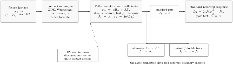
The ODE connection problem determines $\alpha$ and $\beta$. The action and counterterm layer converts $\beta$ into the renormalized canonical momentum. A finite contact term changes the analytic background and generic zeros, but not a nonzero Laurent principal part. Alternate or mixed gates change the source itself and therefore define a different spectral problem.

Normalization covariance

If

$$B_- \longmapsto uB_-, \qquad B_+ \longmapsto vB_+,$$

then $\alpha\mapsto\alpha/u$ and $\beta\mapsto\beta/v$. The quotient changes unless the source and operator normalizations are transformed with it. This is not a defect: a two-point function depends on the normalization of its operator. Its pole set is unchanged when $u$ and $v$ are holomorphic and nowhere zero.

Rescaling the horizon vector by a holomorphic unit $h(\omega)$ multiplies both $\alpha$ and $\beta$ by $h$. It changes neither $\beta/\alpha$ nor the simple-pole residue $\beta(\omega_n)/\alpha'(\omega_n)$.

Local counterterms do not change nonlocal spectral data

A finite quadratic boundary functional has the schematic form

$$S_{\mathrm{fin}} = \frac12 \int\dd^dx\,\sqrt{-g_{(0)}}\, \alpha\, \mathcal P(\Box_{(0)},R_{(0)},\ldots)\alpha.$$

On a flat stationary background it adds a momentum polynomial:

$$G_{\mathrm R} \longmapsto G_{\mathrm R}+P_{\mathrm{loc}}(\omega,\boldsymbol q).$$

It follows that:

• an isolated pole and its Laurent residue are unchanged;
• a nonlocal branch discontinuity is unchanged;
• the analytic real background is scheme dependent;
• a generic zero of the full correlator moves with the scheme;
• changing a logarithmic scale shifts a local polynomial whose anomaly coefficient is fixed.

If $G=N/D+P_{\mathrm{loc}}$ and $D(\omega_n)=0$, combining the fractions adds $P_{\mathrm{loc}}D$ to the numerator. This vanishes at $\omega_n$ and cannot cancel a nonzero principal part.

Counterterms are ultraviolet data. At finite temperature, the divergent ones are the same local covariant functionals as at zero temperature for the same asymptotic theory. Temperature enters the nonlocal coefficient selected by the interior solution.

A contact scheme is not a mixed boundary condition

Adding $P_{\mathrm{loc}}$ leaves the source $\alpha$ fixed. A Robin or multi-trace boundary condition replaces $\alpha$ by a new source functional. The latter changes the theory and can move its poles. Grouping both operations under “boundary counterterms” erases a physical distinction.

Resonant boundaries require a logarithmic canonical pair

For an asymptotically even scalar expansion, a positive integer $\nu=k$ makes the local recursion collide with the fast weight. The boundary series becomes

$$\begin{aligned} \Phi ={}& z^{\Delta_-} \sum_{j=0}^{k-1}z^{2j}\phi_{(2j)} \\ &+ z^{\Delta_+} \left[ \beta_\mu +\psi_{(2k)}\log(z^2\mu^2) +\cdots \right]. \end{aligned}$$

On a flat boundary,

$$\psi_{(2k)} = -\frac{\Box_{(0)}^k\alpha} {4^k k!(k-1)!}.$$

The logarithmic coefficient is locally determined by the source; it is not a third integration constant. Keeping the bulk field fixed while changing the renormalization scale gives

$$\beta_{\mu'} = \beta_\mu -2\psi_{(2k)} \log\frac{\mu'}{\mu}.$$

The renormalized resonant pair is

$$J_k=\alpha, \qquad \sigma_{k,\mu} = 2k\mathcal N_{\mathrm{eff}}\,\beta_\mu +\mathcal L_\mu\alpha,$$

and hence

$$G_{\mathrm R} = 2k\mathcal N_{\mathrm{eff}} \frac{\delta\beta_\mu}{\delta\alpha} +P_\mu.$$

Changing $\mu$ changes only a local polynomial of degree $k$ in momentum squared, or derivative order $2k$. The nonlocal pole ladder remains.

At the Breitenlohner–Freedman point $\nu=0$, both powers coalesce:

$$\Phi = z^{d/2} \left[ \alpha_{\log}\log(z^2\mu^2) +\beta_\mu+\cdots \right].$$

For the displayed normalization, standard BF quantization takes $J_{\mathrm{BF}}=\alpha_{\log}$. In addition to the leading mass counterterm, the regulated action needs the inverse-log subtraction

$$S_{\mathrm{ct}}^{\mathrm{BF}} = -\frac{\mathcal N_\Phi}{2L} \int_{z=\epsilon}\dd^dx\,\sqrt{-\gamma}\, \left[ \frac d2+ \frac{2}{\log(\epsilon^2\mu^2)} \right]\Phi^2+\cdots.$$

Its renormalized canonical partner can be read directly from

$$\langle\mathcal O\rangle_{\mathrm{BF}} = \frac{1}{\sqrt{-g_{(0)}}} \lim_{\epsilon\to0} \epsilon^{d/2}\log(\epsilon^2\mu^2)\, \Pi_{\mathrm{ren}}.$$

It is

$$\sigma_{\mathrm{BF}} = -2\mathcal N_{\mathrm{eff}}\,\beta_\mu +\mathcal L_{\mathrm{loc}}\alpha_{\log}.$$

Keeping the bulk field fixed while changing scale gives

$$\beta_{\mu'} = \beta_\mu -2\alpha_{\log}\log\frac{\mu'}{\mu}.$$

Finite terms suppressed by two inverse logarithms generate the local $\alpha_{\log}$ ambiguity.

Choosing the constant coefficient instead as the source describes a different, generally running mixed theory. Thus one must declare the logarithmic canonical pair; substituting $\nu=0$ into $2\nu\beta/\alpha$ is not a valid limiting prescription.

Standard, alternate, and mixed theories

For the Legendre-transform formulas in this section, freeze the canonical finite scheme by setting $\mathcal L_{\mathrm{loc}}=0$. Independent local functionals may be added afterward; they act by the corresponding fractional-linear change of the response. The canonical standard pair is

$$J_+=\alpha, \qquad \sigma_+ = 2\nu\mathcal N_{\mathrm{eff}}\beta.$$

Alternate quantization is available for a scalar, absent extra exceptional structure, only in the strict window

$$0<\nu<1.$$

Legendre transform the renormalized action:

$$S_- = S_+ -\int\dd^dx\,\sqrt{-g_{(0)}}\, J_+\sigma_+.$$

Then

$$J_-=\sigma_+, \qquad \sigma_-=-J_+,$$

and, in this canonical normalization and before adding independent contact terms,

$$G_-=-G_+^{-1}.$$

In a general standard scheme, $\sigma_+^P=2\nu\mathcal N_{\mathrm{eff}}\beta+P\alpha$, and the same Legendre transform gives $G_-^P=-(G_+^P)^{-1}$. Because $\sigma_+^P$ is then the alternate source, adding $P$ before the transform can move alternate poles. That operation is distinct from adding an independent alternate-theory contact term after the inversion.

Thus a standard response zero may become an alternate pole. Using raw $\beta$, rather than $\sigma_+$, as the alternate source inserts extra factors of $2\nu\mathcal N_{\mathrm{eff}}$; this accounts for many apparent reciprocal-formula disagreements.

For a quadratic large-$N$ multi-trace deformation in the contact-free canonical scheme, take

$$S_f = S_+ +\frac f2 \int\dd^dx\,\sqrt{-g_{(0)}}\,\sigma^2.$$

Its variation is $\delta S_f=\int\sqrt{-g_{(0)}}\,\sigma\,\delta J_f$, which defines

$$J_f = \alpha+f\sigma.$$

Linear response then gives

$$G_f^{\mathrm R} = \left[ (G_0^{\mathrm R})^{-1}+f \right]^{-1} = \frac{G_0^{\mathrm R}} {1+fG_0^{\mathrm R}}.$$

At zero external source, the mixed mode condition is $\alpha+f\sigma=0$. The poles of the deformed theory therefore solve a new boundary equation. With $\sigma=2\nu\mathcal N_{\mathrm{eff}}\beta$, the Robin convention $\beta=\kappa\alpha$ used on the preceding page has

$$\kappa = -\frac{1}{2\nu\mathcal N_{\mathrm{eff}}f}.$$

Reversing the sign in the definition of $J_f$ reverses the sign of $f$; a bare Robin constant is meaningless until this variational and normalization convention is supplied.

A pole audit needs the numerator and the observable

At a simple standard scalar QNM,

$$\alpha(\omega_n,\boldsymbol q)=0, \qquad \partial_\omega\alpha(\omega_n,\boldsymbol q)\ne0,$$

the residue is

$$\operatorname*{Res}_{\omega=\omega_n}G_{\mathrm R} = 2\nu\mathcal N_{\mathrm{eff}} \frac{\beta(\omega_n,\boldsymbol q)} {\partial_\omega\alpha(\omega_n,\boldsymbol q)}.$$

If an angular accessory value $A_{\ell m}(\omega)$ has already been eliminated, the derivative follows that physical sheet:

$$\frac{\dd}{\dd\omega} = \partial_\omega +\frac{\dd A_{\ell m}}{\dd\omega}\partial_A.$$

For a genuine two-vector boundary basis, $\alpha=\beta=0$ would make the solution identically zero. A unique nonzero ingoing scalar line therefore has $\beta(\omega_n)\ne0$ at an ordinary source zero. A simple source zero is a genuine pole; an analytic contact term cannot remove it.

More generally, write the nonlocal part as

$$\frac{N(\omega)}{D(\omega)}, \qquad \begin{aligned} N&\sim(\omega-\omega_*)^q, \\ D&\sim(\omega-\omega_*)^p. \end{aligned}$$

The result has a pole of order $p-q$ if $p>q$, a removable limit if $p=q$, and a zero of order $q-p$ if $q>p$. Common Gamma prefactors, singular basis choices, or observable projectors can manufacture numerator factors that are absent from the primitive connection coordinates.

Coupled fields can hide a collective pole

After constraints and pure-gauge directions have been removed, let the columns of $\mathsf H_{\mathrm{in}}$ be independent physical ingoing solutions. Near the boundary, write

$$\mathsf H_{\mathrm{in}} = B_-\mathsf A+B_+\mathsf B+\cdots.$$

The source-normalized solution matrix is $\mathsf H_{\mathrm{in}}\mathsf A^{-1}$, and the renormalized correlator has the form

$$\mathsf G_{\mathrm R} = \mathsf M\mathsf B\mathsf A^{-1} +\mathsf P_{\mathrm{loc}}.$$

The matrix $\mathsf M$ comes from the quadratic action and the asymptotic symplectic pairing. Derivative mixing can require the more general flux matrix, but the source-matrix logic is unchanged. Collective QNMs satisfy

$$\det\mathsf A(\omega,\boldsymbol q)=0.$$

Suppose a simple rank-one zero has right and left null vectors

$$\mathsf A_n v=0, \qquad u^{\mathsf T}\mathsf A_n=0,$$

and

$$d_n = u^{\mathsf T} (\partial_\omega\mathsf A)_n v \ne0.$$

Then

$$\mathsf A^{-1} = \frac{v u^{\mathsf T}} {(\omega-\omega_n)d_n} +O(1),$$

so

$$\operatorname*{Res}_{\omega_n}\mathsf G_{\mathrm R} = \frac{ \mathsf M_n\mathsf B_n v u^{\mathsf T} }{d_n}.$$

An entry $(i,j)$ has no pole if either $(\mathsf M_n\mathsf B_n v)_i=0$ or $u_j=0$. The QNM still exists in the collective source problem; that particular source or measured operator does not couple to it. If $d_n=0$, the simple-pole formula fails and the next page’s exceptional-point analysis is required.

For gauge fields and gravity, one must first impose radial constraints and use gauge-invariant sources. Ward identities make raw Lorentz-component matrices rank deficient, so their determinant is not a QNM function. A kinematic projector may also make a residue vanish in one component—for example, a diffusive density residue is proportional to $\boldsymbol q^2$ and disappears at zero momentum.

Keep pole-skipping separate

A nonunique horizon line can make both source and response underdetermined at one $(\omega,\boldsymbol q)$. That is not an ordinary cancellation in a unique quotient. Pole-skipping, multiple-mode collisions, exceptional points, and extremal cuts are analyzed systematically on the next page.

KMS reconstructs the equilibrium thermal two-point family

Define

$$\begin{aligned} G^>(t)&=\langle\mathcal O(t)\mathcal O^\dagger(0)\rangle, \\ G^<(t)&=\langle\mathcal O^\dagger(0)\mathcal O(t)\rangle, \\ \rho(\omega)&=-2\operatorname{Im}G_{\mathrm R}(\omega). \end{aligned}$$

For a neutral Hermitian bosonic operator, $\mathcal O^\dagger=\mathcal O$, in equilibrium,

$$\begin{aligned} G^>(\omega) &= [1+n_B(\omega)]\rho(\omega), \\ G^<(\omega) &= n_B(\omega)\rho(\omega), \\ n_B(\omega) &= \frac{1}{\ee^{\omega/T}-1}. \end{aligned}$$

Equivalently,

$$G^>(\omega) = \ee^{\omega/T}G^<(\omega).$$

For a rotating or charged grand-canonical ensemble, keep the $\mathcal O_Q$–$\mathcal O_Q^\dagger$ ordering displayed above and use $\widetilde\omega=\omega-m\Omega-Q\Phi$ in the Bose factor, where $Q$ is the operator charge in a declared gauge. KMS supplies the Wightman and symmetrized functions once $G_{\mathrm R}$ is known. The Matsubara poles of the Bose or $\coth$ factor are thermal-kinematic singularities, not black-hole QNMs.

A stable retarded function is analytic in the upper half of the $\omega$ plane. Damped QNMs lie below the real axis. Their residues control pieces of the time response, but a global QNM sum additionally requires control of large arcs, analytic subtractions, branch cuts, and convergence. Extremal and zero-temperature limits are especially prone to cut formation.

Rotating BTZ gives the exact source/response quotient

Set the AdS radius to one and assume a nonextremal black hole, $r_+>r_-\geq0$. Consider

$$\dd s^2 = -N^2\dd t^2 +\frac{\dd r^2}{N^2} +r^2(\dd\phi+N^\phi\dd t)^2,$$

where

$$\begin{aligned} N^2 &= \frac{(r^2-r_+^2)(r^2-r_-^2)}{r^2}, \\ N^\phi &= -\frac{r_+r_-}{r^2}. \end{aligned}$$

The useful temperatures and horizon angular velocity are

$$\begin{aligned} T_L&=\frac{r_+-r_-}{2\pi}, &T_R&=\frac{r_++r_-}{2\pi}, \\ T_H&=\frac{r_+^2-r_-^2}{2\pi r_+}, &\Omega_H&=\frac{r_-}{r_+}. \end{aligned}$$

For $\Phi=\ee^{-\ii\omega t+\ii k\phi}R(r)$, with $k\in\mathbb Z$, set

$$z = \frac{r^2-r_+^2}{r^2-r_-^2}, \qquad D=r_+^2-r_-^2.$$

The horizon is $z=0$ and the boundary is $z=1$, with

$$1-z = \frac{D}{r^2}+O(r^{-4}).$$

For

$$\nu=\sqrt{1+m^2}, \qquad h=\frac{1+\nu}{2},$$

define

$$q_L = \frac{\omega-k}{4\pi T_L}, \qquad q_R = \frac{\omega+k}{4\pi T_R}.$$

Their sum is the horizon frequency in dimensionless form:

$$q_L+q_R = \frac{\omega-k\Omega_H}{2\pi T_H}.$$

A future-ingoing solution is

$$R_{\mathrm{in}} = z^{-\ii(q_L+q_R)/2} (1-z)^{1-h} {}_2F_1(a,b;c;z),$$

with

$$\begin{aligned} a&=1-h-\ii q_R, \\ b&=1-h-\ii q_L, \\ c&=1-\ii(q_L+q_R). \end{aligned}$$

This hypergeometric representative is a generic horizon chart. When $c\in\mathbb Z_{\leq0}$, its normalization is singular and the ingoing line must be defined by a regularized limit (or by a different local basis). The retarded quotient below is its meromorphic continuation. The extremal limit $r_+\to r_-$ is separate: $z$ and $T_L$ degenerate and a confluent near-horizon problem replaces this chart.

Since $c-a-b=\nu$, Euler’s connection formula gives the slow and fast $z$-chart coefficients

$$\begin{aligned} \alpha_z &= \frac{\Gamma(c)\Gamma(\nu)} {\Gamma(h-\ii q_L)\Gamma(h-\ii q_R)}, \\ \beta_z &= \frac{\Gamma(c)\Gamma(-\nu)} {\Gamma(1-h-\ii q_L)\Gamma(1-h-\ii q_R)}. \end{aligned}$$

Because the physical basis is normalized in powers of $r$, not $1-z$, write

$$R_{\mathrm{in}} = \alpha\,r^{\Delta-2} \left(1+O(r^{-2})\right) + \beta\,r^{-\Delta} \left(1+O(r^{-2})\right), \qquad \Delta=2h.$$

The conversion $1-z\sim D/r^2$ gives

$$\alpha=D^{1-h}\alpha_z, \qquad \beta=D^h\beta_z,$$

and hence

$$\frac{\beta}{\alpha} = D^\nu\frac{\beta_z}{\alpha_z}.$$

For noninteger $\nu$, away from a coincident Gamma pole–zero locus, the correlator in the declared normalization is therefore

$$\begin{aligned} G_{\mathrm R}^{\mathrm{BTZ}} ={}& 2\nu\mathcal N_\Phi D^\nu \frac{\Gamma(-\nu)}{\Gamma(\nu)} \\ &\times \frac{ \Gamma(h-\ii q_L)\Gamma(h-\ii q_R) }{ \Gamma(1-h-\ii q_L) \Gamma(1-h-\ii q_R) } +P_{\mathrm{loc}}. \end{aligned}$$

At generic points, the two source-zero ladders are

$$\begin{aligned} \omega_n^{(L)} &= k-4\pi\ii T_L(n+h), \\ \omega_n^{(R)} &= -k-4\pi\ii T_R(n+h), \qquad n=0,1,2,\ldots. \end{aligned}$$

They are precisely the rotating-BTZ scalar QNMs. For $T_L,T_R,h>0$ they lie in the lower half-plane. Denominator-Gamma poles are zeros of this minimal nonlocal quotient, but adding $P_{\mathrm{loc}}$ moves zeros of the full correlator. If a source-zero condition meets a response-zero condition, the apparent pole and zero must be resolved in the full two-parameter limit; these exceptional intersections are the elementary Gamma-function model of pole-skipping. Likewise, $c\in\mathbb Z_{\leq0}$ requires the regularized horizon normalization just described. An expression written as $|\Gamma|^2$ on the real axis must not be used for analytic continuation in complex $\omega$; the holomorphic Gamma quotient above is the spectral object.

The massless scalar exposes the logarithmic subtraction

At $m^2=0$, $\nu=1$ and $h=1$. Direct substitution into the preceding formula is illegal because $\Gamma(-\nu)$ diverges while the boundary basis becomes logarithmic. Define

$$p_+=\frac{\omega-k}{2}, \qquad p_-=\frac{\omega+k}{2}.$$

Regulate with $\nu=1+\varepsilon$ and replace $D^\nu$ by $D^\nu\mu^{-2\varepsilon}$. After subtracting the local pole, the nonlocal content in the action normalization fixed above is

$$\begin{aligned} G_{\mathrm R}^{\mathrm{ren}} ={}& -2\mathcal N_\Phi\,p_+p_- \biggl[ \psi\!\left( 1-\frac{\ii p_+}{2\pi T_L} \right) \\ &\qquad+ \psi\!\left( 1-\frac{\ii p_-}{2\pi T_R} \right) +\log\frac{D}{\mu^2} \biggr] +P_{\mathrm{fin}}. \end{aligned}$$

Here $P_{\mathrm{fin}}$ collects the remaining analytic part fixed by the chosen continuation together with any optional finite local scheme term; only the latter is freely adjustable. Changing $\mu$ shifts a local multiple of $p_+p_-=(\omega^2-k^2)/4$. The digamma poles retain the two QNM towers with $h=1$. This is a concrete example in which the infinity of a raw Gamma factor is a renormalization artifact while the thermal pole ladder is finite.

An exact source-free micro-mode

Take

$$r_+=1, \qquad r_-=0, \qquad m^2=-\frac34, \qquad k=1.$$

Then $T_L=T_R=1/(2\pi)$, $\nu=1/2$, and $h=3/4$. At

$$\omega_*=1-\frac32\ii,$$

one finds

$$q_L=-\frac34\ii, \qquad q_R=1-\frac34\ii, \qquad a=c=-\frac12-\ii, \qquad b=-\frac12.$$

The identity

$${}_2F_1(c,b;c;z) =(1-z)^{-b}$$

therefore gives

$$R_{\mathrm{in}} = z^{-\ii(q_L+q_R)/2}(1-z)^h.$$

It is purely fast at the boundary: $\alpha_z=0$ and $\beta_z=1$. This checks the lowest left QNM without root finding and confirms directly that its response coefficient does not vanish.

A Heun recurrence changes the engine, not the ledger

In higher-dimensional charged AdS black holes, the radial equation is generically Heun rather than hypergeometric. As one example, the scalar equation in a five-dimensional Reissner–Nordström–AdS family can be mapped with

$$z = \frac{r^2-r_+^2}{r^2-r_-^2}$$

to a four-regular-singularity connection problem. Use dimensionless AdS units $L=1$, assume the nonextremal generic chart $|t|>1$, and let $r_0^2$ denote the remaining root of the blackening polynomial. Ren and Yu use

$$\begin{aligned} t &= \frac{r_0^2-r_+^2}{r_0^2-r_-^2}, \qquad |t|>1, \\ \phi &= z^{-1/2}(1-z)^{1/2} \left(1-\frac zt\right)^{-1/2}\psi. \end{aligned}$$

The common gauge factor does not alter the coefficient ratio, but it must be undone before assigning physical boundary powers. Normalize the canonical Heun source and response bases to unit leading coefficients in their $(1-z)$ powers. Let

$$D_R=r_+^2-r_-^2, \qquad \nu_4=\sqrt{4+m^2}.$$

On a generic nonresonant chart, abbreviate the suppressed monodromy and accessory data by

$$\begin{aligned} C_\pm &= C(\theta_0,\pm\theta_1; t,\theta_t,\theta_\infty,w), \\ \theta_0&=\frac{\ii\omega}{4\pi T_+}, &\theta_1&=\frac{\nu_4}{2}. \end{aligned}$$

The exact canonical-Heun connection formula is

$$\psi_{\mathrm{in}} = C_+\psi_{\mathrm{src}} +C_-\psi_{\mathrm{resp}}.$$

The displayed $\theta_0$ is for a neutral scalar in the horizon-regular gauge. A charged mode uses the corresponding covariant horizon frequency.

After undoing the common gauge, its finite factor $(1-1/t)^{-1/2}$ cancels between the two coefficients. Converting the unit $(1-z)$ powers to the unit-leading physical $r$-basis with $1-z\sim D_R/r^2$ gives the holographic quotient

$$\frac{\beta}{\alpha} = D_R^{\nu_4} \frac{C_-}{C_+}.$$

A three-term recurrence can compute $C$. Holography still requires

$$G_{\mathrm R} = 2\nu_4\mathcal N_\Phi D_R^{\nu_4} \frac{C_-}{C_+} +P_{\mathrm{loc}}.$$

Thus a recurrence formula quoted “up to a prefactor” is sufficient for generic QNM locations, but not for normalized residues, contact terms, or the real analytic background. When $m=0$, $\nu_4=2$: the boundary is resonant, and the logarithmic connection matrix and counterterms must replace the generic quotient. Ren and Yu’s published tables show mode-by-mode agreement with independent pseudospectral calculations over many digits in their stated RN–AdS$_5$ benchmarks. That agreement validates the connection engine, not an omitted normalization ledger.

A reproducible correlator workflow

1. Freeze the bulk convention. Record the quadratic action, Fourier sign, radial field, gauge, and operator normalization.
2. Select the causal horizon line. Construct it in future-regular coordinates and continue from the upper half-plane.
3. Build the ultraviolet canonical pair. Include logarithms and scale data on resonant strata.
4. Compute primitive connection coefficients. Use Wronskians, recurrence minimality, direct integration, or an exact connection formula.
5. Renormalize the canonical momentum. Derive divergent counterterms from local ultraviolet recursion and state the finite scheme.
6. Declare the boundary theory. Choose standard, alternate, or a normalized mixed variational problem.
7. Audit poles and residues. Check the source zero, numerator order, observable projection, constraints, and derivative along any accessory sheet.
8. Cross-check independently. Compare match points and precisions, use a second solver, test reality and upper-half-plane analyticity, and evaluate the original boundary function at every candidate pole.

Common pitfalls

Calling $\beta/\alpha$ a fully normalized correlator. The quotient is connection data. The kinetic normalization, the factor $2\nu$, logarithmic subtractions, and finite local terms come from the renormalized action.

Using an outgoing branch with $\ee^{-\ii\omega t}$. A retarded solution is regular in $v=t+r_*$ and carries the radial factor $\ee^{-\ii\omega r_*}$. At complex frequency, define it by causal analytic continuation.

Reading the response from an arbitrary transformed field. The observable is conjugate to the source under variation of the complete renormalized action. A Schrödinger gauge or Heun gauge may insert powers and boundary factors that must be undone.

Treating a resonant logarithm as an ordinary second power. At integer $\nu$, the logarithmic coefficient is locally fixed by the source and the free fast coefficient depends on $\mu$. Use the renormalized log-adapted pair.

Calling correlator zeros scheme independent. A finite local polynomial moves generic zeros. A primitive source zero, a collective source-matrix zero, and a zero of a chosen full correlator are different objects.

Using alternate quantization outside its window. A formal exchange of coefficients does not establish a normalizable unitary boundary theory.

Calling a double-trace pole shift a contact ambiguity. A double-trace term changes the source functional and the mode equation. A finite source counterterm does not.

Taking the determinant before removing gauge directions. Constraints and Ward identities make raw source matrices singular. Build a square physical source map first.

Exercises

1. Derive the first scalar counterterms

Starting from the displayed bulk action, derive $\Pi_\epsilon$ and $S_{\mathrm{reg}}^{\mathrm{os}}=\frac12\int\Phi\Pi_\epsilon$. Substitute

$$\Phi = z^{\Delta_-} \left(\alpha+z^2\phi_{(2)}+\cdots\right)$$

into the Klein–Gordon equation and show that

$$\phi_{(2)} = \frac{\Box_{(0)}\alpha}{4(\nu-1)}.$$

Verify that $S_{\mathrm{ct}}^{(0)}+S_{\mathrm{ct}}^{(2)}$ cancels the first two power divergences when $\nu>1$.

Solution

Integration by parts produces the outward-normal term $-\mathcal N_\Phi\sqrt{-\gamma}\,n\cdot\partial\Phi$, which is $\Pi_\epsilon$. The indicial polynomial is $P(\lambda)=\lambda(\lambda-d)-m^2L^2$. At the next weight,

$$P(\Delta_-+2) = -4(\nu-1).$$

The coefficient equation $P(\Delta_-+2)\phi_{(2)}+\Box_{(0)}\alpha=0$ gives the claimed result. The leading term in $S_{\mathrm{reg}}^{\mathrm{os}}$ is canceled by $S_{\mathrm{ct}}^{(0)}$; the remaining $z^{2-2\nu}\alpha\Box_{(0)}\alpha$ term is canceled by $S_{\mathrm{ct}}^{(2)}$. At $\nu=1$, the latter power becomes a logarithm.

2. Recover the Wronskian quotient

Starting from $R_H^{\mathrm{in}}=\alpha B_-+\beta B_+$, derive the two Wronskian formulas and prove

$$\frac{\beta}{\alpha} = \frac{E_{\mathrm{alt}}}{E_{\mathrm{std}}}.$$

Show that the result is independent of the match point.

Solution

Taking $\mathcal W[\,\cdot\,,B_+]$ kills the $B_+$ term and gives $\alpha\mathcal W[B_-,B_+]$. Taking $\mathcal W[B_-,\,\cdot\,]$ kills the $B_-$ term and gives $\beta\mathcal W[B_-,B_+]$. Their ratio is the displayed quotient. Abel’s identity makes every weighted Wronskian constant on a connected overlap, and the common factor $W_0$ cancels between $E_{\mathrm{alt}}$ and $E_{\mathrm{std}}$.

3. Prove that contact terms preserve a pole

Let

$$G(\omega) = \frac{N(\omega)}{D(\omega)}+P(\omega),$$

where $P$ is analytic at a simple zero $D(\omega_n)=0$ and $N(\omega_n)\ne0$. Prove that the pole position and residue are unchanged, and explain why a generic zero of $G$ is not protected.

Solution

Combining fractions gives

$$G = \frac{N+PD}{D}.$$

At $\omega_n$, the new numerator is still $N(\omega_n)$, so the residue is $N(\omega_n)/D'(\omega_n)$. Away from a pole, the equation $N+PD=0$ depends explicitly on $P$, so its roots move under a finite scheme change.

4. Derive alternate and double-trace response

Vary

$$S_-=S_+-\int J_+\sigma_+$$

and show that $G_-=-G_+^{-1}$. Then use $\delta J_f=\delta\alpha+f\delta\sigma$ to derive

$$G_f=(G_0^{-1}+f)^{-1}.$$

Why does the old pole of $G_0$ generally cease to be a pole of $G_f$?

Solution

Because $\delta S_+=\int\sigma_+\delta J_+$,

$$\delta S_- = -\int J_+\delta\sigma_+.$$

Thus $J_-=\sigma_+$ and $\sigma_-=-J_+$, giving $G_-=-G_+^{-1}$. For the mixed source, $\delta\sigma=G_0\delta\alpha$ and

$$\delta J_f = (G_0^{-1}+f)\delta\sigma.$$

Inverting yields the formula. If $G_0\to\infty$, then $G_f\to1/f$; the new poles instead solve $1+fG_0=0$.

5. Find the rotating-BTZ QNM towers

Assume $c\notin\mathbb Z_{\leq0}$ and no cross-sector Gamma pole–zero intersection. Use Euler’s connection formula to derive $\alpha_z$ and $\beta_z$. Then locate the zeros of $\alpha_z$ and obtain both QNM ladders. Explain why the excluded intersections require a limiting analysis.

Solution

The two coefficients in the $z\to1$ connection formula are

$$\frac{\Gamma(c)\Gamma(c-a-b)} {\Gamma(c-a)\Gamma(c-b)}$$

and

$$\frac{\Gamma(c)\Gamma(a+b-c)} {\Gamma(a)\Gamma(b)}.$$

Using $c-a-b=\nu$, $c-a=h-\ii q_L$, and $c-b=h-\ii q_R$ gives the displayed $\alpha_z$ and $\beta_z$. Because $\Gamma$ has poles but no zeros, and because the excluded genericity conditions prevent an indeterminate product, $\alpha_z=0$ when $h-\ii q_L=-n$ or $h-\ii q_R=-n$. Solving these equations gives

$$\omega_n^{(L)} = k-4\pi\ii T_L(n+h),$$

and

$$\omega_n^{(R)} = -k-4\pi\ii T_R(n+h).$$

If a left numerator pole meets a right denominator pole, then $c=-n-m\in\mathbb Z_{\leq0}$; the chosen horizon representative is singular at precisely that intersection. One must regularize the ingoing basis and take the joint parameter limit, as in the pole-skipping analysis on the next page.

6. Take the massless BTZ limit correctly

Set $\nu=1+\varepsilon$ in the regulated factor $D^\nu\mu^{-2\varepsilon}$. Show that its $1/\varepsilon$ term is a local multiple of $p_+p_-$ and that the finite nonlocal part is $-2\mathcal N_\Phi p_+p_-$ times the displayed digamma sum.

Solution

Use

$$\Gamma(-1-\varepsilon) = \frac{1}{\varepsilon}+O(1)$$

and differentiate the four Gamma functions with respect to $\nu$, remembering that $h=(1+\nu)/2$. At $\varepsilon=0$,

$$\frac{\Gamma(h-\ii q)} {\Gamma(1-h-\ii q)} = -\ii q.$$

The product $D(-\ii q_L)(-\ii q_R)=-p_+p_-$ makes the divergent term a local polynomial. The finite derivative produces $\psi(1-\ii q_L)+\psi(1-\ii q_R)$ plus constants and $\log(D/\mu^2)$. Restoring the prefactor gives the declared coefficient $-2\mathcal N_\Phi$. Rational differences contribute analytic terms; together with optional local finite counterterms they are recorded in $P_{\mathrm{fin}}$, but only the counterterm part is scheme adjustable.

7. Derive the coupled-field residue

Assume $\mathsf A_n v=0$, $u^{\mathsf T}\mathsf A_n=0$, and $u^{\mathsf T}\mathsf A_n'v\ne0$. Prove the rank-one Laurent formula for $\mathsf A^{-1}$ and give a $2\times2$ example in which one correlator entry does not see the pole.

Solution

Insert

$$\mathsf A^{-1} = \frac{\mathsf R}{\omega-\omega_n}+O(1)$$

into $\mathsf A\mathsf A^{-1}=\mathsf I$. The leading equation implies that the image of $\mathsf R$ lies in $\operatorname{span}(v)$ and its row space lies in $\operatorname{span}(u^{\mathsf T})$. The finite equation fixes

$$\mathsf R = \frac{v u^{\mathsf T}} {u^{\mathsf T}\mathsf A_n'v}.$$

For example, take

$$\mathsf A = \begin{pmatrix} 1&0\\ 0&\omega-\omega_n \end{pmatrix}, \qquad \mathsf M\mathsf B = \begin{pmatrix} 1&0\\ 0&1 \end{pmatrix}.$$

Only the $(2,2)$ entry has a pole. The collective source determinant still vanishes at $\omega_n$.

8. Audit the exact BTZ micro-mode

For the parameters in the details box, verify $a=c$, use ${}_2F_1(c,b;c;z)=(1-z)^{-b}$, and show directly that the solution is future-ingoing and purely fast at the boundary.

Solution

Substitution gives

$$a=c=-\frac12-\ii, \qquad b=-\frac12.$$

The hypergeometric factor contributes $(1-z)^{1/2}$, so the total boundary power is $(1-z)^{1-h+1/2}=(1-z)^h$. The slow coefficient vanishes and the fast coefficient is one. The factor $z^{-\ii(q_L+q_R)/2}$ is the declared future-ingoing horizon factor.

References

• S. de Haro, K. Skenderis, and S. N. Solodukhin, “Holographic Reconstruction of Spacetime and Renormalization in the AdS/CFT Correspondence”, Communications in Mathematical Physics 217 (2001), 595–622. Derives the covariant counterterm algorithm and the nonlocal $(2\Delta-d)$ response coefficient plus local source terms.
• K. Skenderis, “Lecture Notes on Holographic Renormalization”, Classical and Quantum Gravity 19 (2002), 5849–5876. Develops scalar recursion, logarithmic anomalies, renormalized one-point functions, and contact-term scheme dependence.
• A. Karch, A. O’Bannon, and K. Skenderis, “Holographic Renormalization of Probe D-Branes in AdS/CFT”, JHEP 04 (2006), 015. Gives an explicit scalar Breitenlohner–Freedman-bound treatment with the inverse-log counterterm and logarithmic source prescription.
• D. T. Son and A. O. Starinets, “Minkowski-Space Correlators in AdS/CFT Correspondence: Recipe and Applications”, JHEP 09 (2002), 042. Gives the future-ingoing prescription, thermal relations, the exact BTZ correlator, and the response/source explanation of QNM poles.
• K. Skenderis and B. C. van Rees, “Real-Time Gauge/Gravity Duality: Prescription, Renormalization and Examples”, JHEP 05 (2009), 085. Supplies the systematic Schwinger–Keldysh construction and real-time holographic renormalization.
• D. Birmingham, I. Sachs, and S. N. Solodukhin, “Conformal Field Theory Interpretation of Black Hole Quasi-Normal Modes”, Physical Review Letters 88 (2002), 151301. Matches the exact BTZ QNM towers to poles of the thermal CFT retarded function.
• I. R. Klebanov and E. Witten, “AdS/CFT Correspondence and Symmetry Breaking”, Nuclear Physics B 556 (1999), 89–114. Establishes the two scalar quantizations in the admissible mass range and their Legendre-transform relation.
• E. Witten, “Multi-Trace Operators, Boundary Conditions, and AdS/CFT Correspondence”, arXiv:hep-th/0112258. Relates multi-trace deformations to generalized AdS boundary conditions.
• P. Kovtun and A. O. Starinets, “Quasinormal Modes and Holography”, Physical Review D 72 (2005), 086009. Constructs gauge-invariant master fields and relates AdS QNMs to poles of retarded stress-tensor and current correlators.
• M. Kaminski, K. Landsteiner, J. Mas, J. P. Shock, and J. Tarrío, “Holographic Operator Mixing and Quasinormal Modes on the Brane”, JHEP 02 (2010), 021. Develops the matrix-valued flux and source-map formalism for coupled bulk fields and residue matrices.
• N. Iqbal and H. Liu, “Universality of the Hydrodynamic Limit in AdS/CFT and the Membrane Paradigm”, Physical Review D 79 (2009), 025023. Formulates response through the radial canonical momentum and its horizon-to-boundary flow.
• J. Ren and Z. Yu, “Holographic Thermal Correlators from Recursions”, JHEP 06 (2025), 183. Computes Heun horizon-to-boundary connection quotients by recurrence and benchmarks RN–AdS$_5$ QNMs against pseudospectral calculations.