Symanzik Rotations and Anharmonic-Oscillator Prototypes

The preceding page showed that shifting a pair of decay sectors rotates a lateral spectrum, but left a nowhere-zero factor $\chi$ in the corresponding Wronskian. That factor cannot be fixed by sector geometry alone. A rotation changes the independent variable, the energy, every lower coupling, the contour, and the normalization of the canonical solution.

A Symanzik rotation keeps this complete passport. For a homogeneous anharmonic oscillator it acts only on $x$ and $E$, and the normalization used on Pages 1–2 makes the action especially simple. For a general polynomial, one further number matters: the coefficient of $x^{-1}$ in the formal momentum $\sqrt{P(x)-E}$. That coefficient produces a logarithm in the WKB action, hence an algebraic power of $x$ and a computable phase under rotation.

This page derives those phases entirely on the ODE side. It does not yet call an endpoint function a Baxter $Q$-function, identify the centrifugal parameter with a twist, or name a Stokes coefficient as a transfer-matrix eigenvalue. Those are additional dictionaries, beginning on Page 4.

The result to retain

Let

$$P(x)=x^{2M}+\sum_{a=0}^{2M-1}g_a x^a, \qquad M\in\mathbb N, \quad M>1,$$

and set

$$\omega=\exp\left(\frac{\pi\ii}{M+1}\right), \qquad s_k=(-1)^k.$$

If $b$ is the coefficient of $x^{-1}$ in the large-$x$ expansion of $\sqrt{P(x)-E}$, then the adjacent-normalized Symanzik orbit is

$$\begin{aligned} y_k(x;p) ={}& \omega^{k/2-k s_k b(p)} y_0\!\left(\omega^{-k}x;\mathcal R_kp\right), \\ \mathcal R_kp ={}& \left( \omega^{2k}E, \{\omega^{(a+2)k}g_a\}_{a=0}^{2M-1} \right). \end{aligned}$$

With the half-powers and logarithms fixed below,

$$\Wr[y_k,y_{k+1}]=2\ii$$

for every $k$. Moreover,

$$\begin{aligned} \Wr[y_{j+r},y_{k+r}](p) ={}& \omega^{-r b(p)(s_{j+r}+s_{k+r})} \\ &\times \Wr[y_j,y_k](\mathcal R_rp). \end{aligned}$$

This is the normalization-complete version of the Page 2 rotation law.

Status ledger

Statement used on this page	Status
Covariance of the differential equation under $x=\omega^kX$	Exact substitution
Rotation weights of $E$ and the lower polynomial coefficients	Exact algebra
Existence of the canonically normalized recessive solution and its parameter analyticity	Global asymptotic ODE theorem for the stated polynomial family
The logarithmic WKB coefficient and its sign under rotation	Exact formal expansion after a branch at infinity is fixed
The adjacent Wronskian $2\ii$ and the shifted-Wronskian law	Exact consequence of the displayed normalization and canonical asymptotics
Finite scalar return after $2M+2$ steps	Derived here from the normalized orbit and entire continuation for an equation without finite singularities; modified by finite-point monodromy when singularities are present
The six-step quartic parameter orbit	Exact for the displayed polynomial family
Calling the endpoint functions Baxter $Q$-functions or the scalar multiplier a transfer matrix	Model-dependent dictionary, deferred
A truncated fusion hierarchy or a $Y$-system	Additional functional relations and analyticity hypotheses, deferred

Rotation acts on the whole spectral passport

Consider

$$\left[-\frac{\dd^2}{\dd x^2}+P(x)\right]y(x)=E y(x), \qquad P(x)=x^{2M}+\sum_{a=0}^{2M-1}g_a x^a.$$

Put $x=\omega^kX$. Since $\omega^{2(M+1)}=1$, multiplication of the transformed equation by $\omega^{2k}$ restores the leading coefficient:

$$\left[ -\frac{\dd^2}{\dd X^2} +X^{2M} +\sum_{a=0}^{2M-1} \omega^{(a+2)k}g_aX^a \right]y = \omega^{2k}E\,y.$$

Thus the exact action on the parameter passport $p=(E,\{g_a\})$ is

$$\mathcal R_kp = \left( \omega^{2k}E, \{\omega^{(a+2)k}g_a\} \right).$$

The same rule can be indexed from the top of the polynomial. If

$$P(x)=x^{2M}+a_1x^{2M-1}+\cdots+a_{2M},$$

then

$$a_j\longmapsto\omega^{-jk}a_j.$$

These are the same weights because $\omega^{(2M-j+2)k}=\omega^{-jk}$. The constant coefficient and the energy acquire the same weight, and only the combination $g_0-E$ enters the equation. Keeping both is sometimes convenient for a coupling ledger, but one may always be absorbed into the other.

The active and passive descriptions should not be mixed:

• the coordinate change sends the arguments in a canonical solution to $(\omega^{-k}x,\mathcal R_kp)$;
• the physical ends of the contour rotate from $(\mathcal S_j,\mathcal S_m)$ to $(\mathcal S_{j+k},\mathcal S_{m+k})$;
• a spectral zero consequently rotates in the inverse direction when it is expressed in the unrotated energy coordinate.

Rotating $E$ while leaving a nonzero lower coupling fixed is therefore not, in general, a covariance of the same equation.

The logarithmic WKB coefficient fixes the representative

The leading exponential is not the complete normalization datum. Choose the branch of the formal momentum with

$$\sqrt{P(x)-E}\sim x^M$$

in the positive sector. Its expansion has the form

$$\sqrt{P(x)-E} = x^M+c_1x^{M-1}+\cdots+c_M +\frac{b(p)}{x}+O(x^{-2}).$$

Fix the additive constant by defining the positive-power primitive

$$\Phi(x;p) = \frac{x^{M+1}}{M+1} +\sum_{j=1}^{M} \frac{c_jx^{M+1-j}}{M+1-j}.$$

Then

$$\int^x\sqrt{P(t)-E}\,\dd t = \Phi(x;p)+b(p)\log x+O(x^{-1}),$$

The logarithm explains the extra power in the canonical asymptotic. We fix the positive-sector solution by

$$y_0(x;p) \sim x^{-M/2-b(p)} \exp[-\Phi(x;p)]$$

with leading coefficient one. The branch of $\log x$ belongs to this definition. For $M>1$, the spectral term $-E$ first contributes to the formal momentum at order $x^{-M}$, so $b$ is independent of $E$. At the harmonic threshold $M=1$, it contributes directly to $x^{-1}$; that exception will be important below.

We call $b$ the logarithmic WKB coefficient. With the standard coordinate at infinity, the one-form has $\operatorname{Res}_{x=\infty}\sqrt{P(x)-E}\,\dd x=-b$; this sign is why calling $b$ itself a residue can be misleading.

Let $q(x;p)=\sqrt{P(x)-E}$ with the declared branch. Under one rotation, the exact formal covariance is

$$q(X;\mathcal R_kp) = s_k\omega^k q(\omega^kX;p).$$

Because $\Phi$ was assigned zero constant, integration gives

$$\Phi(\omega^{-k}x;\mathcal R_kp) = s_k\Phi(x;p).$$

In particular, coefficient comparison gives

$$b(\mathcal R_kp)=s_k b(p), \qquad s_k=(-1)^k.$$

We use the unambiguous half-power convention

$$\omega^{q} := \exp\left(\frac{q\pi\ii}{M+1}\right)$$

for every exponent $q$ that appears below. Define

$$y_k(x;p) = \omega^{k/2-k s_k b(p)} y_0\!\left(\omega^{-k}x;\mathcal R_kp\right).$$

The transformed function solves the original equation with passport $p$ and is recessive in $\mathcal S_k$. More importantly, its leading term is

$$\begin{aligned} y_k(x;p) \sim{}& \ii^k x^{-M/2-s_kb(p)} \\ &\times \exp\left[-s_k\Phi(x;p)\right], \end{aligned}$$

The prefactor has been chosen so that the printed coefficient is exactly $\ii^k$; it is not decorative.

In a common enlarged asymptotic wedge,

$$\begin{aligned} y_k' &\sim-s_kx^M y_k, & y_{k+1}' &\sim s_kx^M y_{k+1}. \end{aligned}$$

The two algebraic powers multiply to $x^{-M}$, and hence

$$\begin{aligned} \Wr[y_k,y_{k+1}] &= 2s_k\ii^k\ii^{k+1} \\ &=2\ii. \end{aligned}$$

The asymptotic calculation determines the constant Wronskian everywhere by Abel’s identity. It also explains a common convention mismatch. If one uses only the factor $\omega^{k/2}$ for a polynomial with $b\ne0$, the rotated solutions still span the correct recessive lines, but their adjacent Wronskians carry formal-monodromy phases. The extra $\omega^{-ks_kb}$ is what makes the Page 2 gauge global.

Two useful specializations

For the homogeneous family $P=x^{2M}$, one has $b=0$ and

$$y_k(x,E) = \omega^{k/2} y_0(\omega^{-k}x,\omega^{2k}E).$$

For the standard one-coefficient deformation

$$P(x)=x^{2M}+\alpha x^{M-1},$$

the formal momentum begins as

$$\sqrt{P(x)-E} = x^M+\frac{\alpha}{2x}+\cdots,$$

so $b=\alpha/2$ and $\alpha$ changes sign at every step. The normalized orbit becomes

$$\begin{aligned} y_k(x,E,\alpha) ={}& \omega^{k/2-k(-1)^k\alpha/2} \\ &\times y_0\!\left( \omega^{-k}x, \omega^{2k}E, (-1)^k\alpha \right). \end{aligned}$$

Many ODE/IM references instead use a leading coefficient $1/\sqrt{2\ii}$. Restoring unit leading coefficient, their standard representatives are

$$Y_k = \omega^{k(1+\alpha)/2} y_0\!\left( \omega^{-k}x, \omega^{2k}E, s_k\alpha \right).$$

The present Page 2 gauge is related to them by

$$y_k = \omega^{-k\alpha(1+s_k)/2}Y_k.$$

The two central adjacent Wronskians of the literature gauge are $2\ii$ after this common rescaling, and its triple $k=-1,0,1$ agrees with the present triple. Farther around the orbit,

$$\Wr[Y_k,Y_{k+1}] = 2\ii\, \omega^{\alpha\left[k+(1-s_k)/2\right]},$$

so the two representative families should not be silently combined. Their returns differ for the same reason:

$$\begin{aligned} Y_{k+N} &=-\ee^{\pi\ii\alpha}Y_k, & y_{k+N} &=-\ee^{-\pi\ii s_k\alpha}y_k. \end{aligned}$$

Rotated Wronskians have an exact phase

Write

$$W_{j,k}(p):=\Wr[y_j,y_k](p).$$

To shift both indices by $r$, put $X=\omega^{-r}x$. Directly from the definition,

$$\begin{aligned} y_{j+r}(x;p) ={}& \omega^{r/2-rs_{j+r}b(p)} \\ &\times y_j(X;\mathcal R_rp). \end{aligned}$$

There is one such factor for each solution and a derivative Jacobian $\dd X/\dd x=\omega^{-r}$. Therefore

$$\begin{aligned} W_{j+r,k+r}(p) ={}& \omega^{-rb(p)(s_{j+r}+s_{k+r})} \\ &\times W_{j,k}(\mathcal R_rp). \end{aligned}$$

This formula evaluates the Page 2 factor $\chi$. For adjacent indices the two signs cancel, recovering $W_{k,k+1}=2\ii$. For the elementary lateral Wronskian $W_{k-1,k+1}$ the indices have the same parity, so the logarithmic phase survives. More generally, that phase survives exactly when the two shifted indices have the same parity.

Define the scalar Stokes coefficient in the frozen Page 2 gauge by

$$C_k(p) = \frac{W_{k-1,k+1}(p)}{2\ii}.$$

Taking $(j,k,r)=(-1,1,k)$ gives

$$C_k(p) = \omega^{2k s_k b(p)} C_0(\mathcal R_kp).$$

For $b=0$ this reduces to the familiar homogeneous relation $C_k(E)=C_0(\omega^{2k}E)$. For the $\alpha$ deformation it reads

$$C_k(E,\alpha) = \omega^{k(-1)^k\alpha} C_0\!\left( \omega^{2k}E, (-1)^k\alpha \right).$$

Both are exact ODE identities. No operator from an integrable model has entered.

At an ordinary origin, the endpoint functionals transform just as explicitly. If

$$A(p)=y_0(0;p), \qquad B(p)=y_0'(0;p),$$

then

$$\begin{aligned} y_k(0;p) &= \omega^{k/2-ks_kb(p)}A(\mathcal R_kp), \\ y_k'(0;p) &= \omega^{-k/2-ks_kb(p)}B(\mathcal R_kp). \end{aligned}$$

These formulas rotate the Dirichlet and Neumann boundary functions of Page 1 without yet assigning them an integrable-model name. Normalize each rotated endpoint function at $E=0$ and write $g^{(k)}$ for the rotated lower couplings. For $B\in\{\mathrm D,\mathrm N\}$,

$$\begin{aligned} D_{B,k}(E;g) ={}& \omega^{-ks_k[b(E,g)-b(0,g)]} \\ &\times D_B(\omega^{2k}E;g^{(k)}). \end{aligned}$$

For $M>1$, $b$ is independent of $E$, and the displayed phase cancels. At $M=1$ it survives. This is the normalized-determinant counterpart of the raw endpoint formulas.

Finite sector return includes formal holonomy

For an even polynomial degree $2M$, the number of Stokes sectors is

$$N=2M+2.$$

The parameter passport returns after $N$ steps and $s_{k+N}=s_k$. If the equation has no finite singularities, direct substitution in the normalized orbit and entire continuation give

$$y_{k+N} = -\exp[-2\pi\ii s_kb(p)]\,y_k.$$

Thus the recessive line closes, but its chosen representative returns with formal holonomy. In the homogeneous case $b=0$,

$$y_{k+N}=-y_k.$$

If the potential is even, the half-turn is also a symmetry. For $P=x^{2M}$,

$$y_{k+M+1}(x,E) = \ii\,y_k(-x,E).$$

These two identities are statements about canonical ODE solutions. A truncation of a fusion hierarchy requires a further dictionary and is not being asserted here. The finite return nevertheless imposes an exact basis identity. Put

$$A_j= \begin{pmatrix} C_j&1\\ -1&0 \end{pmatrix}, \qquad \mu_j=-\ee^{-2\pi\ii s_jb},$$

so that $(y_{j-1},y_j)=(y_j,y_{j+1})A_j$. Iterating once around the sector orbit gives

$$A_{k+N}\cdots A_{k+1} = \begin{pmatrix} \mu_k&0\\ 0&\mu_{k+1} \end{pmatrix}^{-1}.$$

For $b=0$ the product is $-\mathbf 1$. This is finite-dimensional ODE monodromy algebra, not yet a fusion relation.

Two qualifications matter.

A singular origin. Adding $l(l+1)/x^2$ leaves the coefficient invariant under every $\mathcal R_k$, but the origin has exponents $l+1$ and $-l$. Let $\mathcal M_0$ denote positive counterclockwise local monodromy. Since $\omega^{-N}x$ follows the declared clockwise continuation, the return becomes

$$y_{k+N} = -\exp[-2\pi\ii s_kb] \bigl(\mathcal M_0^{-1}\!\cdot y_k\bigr).$$

Away from resonance, the local monodromy eigenvalues are $\ee^{2\pi\ii(l+1)}$ and $\ee^{-2\pi\ii l}$. A canonical solution selected at infinity is generally not one of those eigenvectors, so scalar closure is not automatic. Page 4 replaces evaluation at zero by Frobenius connection coefficients. When $2l+1\in\mathbb Z$, logarithmic Frobenius terms and non-semisimple local monodromy may require a separate resonant analysis.

A genuinely branched power. If $2M\notin\mathbb Z$, then $x^{2M}$ lives on a chosen logarithmic cover. Local rotations remain meaningful there, but $2M+2$ need not be an integer sector count and a projected finite return cannot be imported from the polynomial case. Irrational $M$ has no finite root-of-unity orbit. When $2M$ is an odd integer, the potential is instead an odd-degree polynomial with $2M+2$ sectors, but the present even-degree bookkeeping—including $s_{k+N}=s_k$ and the half-turn discussion—must be rederived for that family.

Page 7 returns to the broader question: which polynomial and exponential families turn local covariance into useful closed functional systems.

The quartic passport closes after six steps

The quartic family makes the different periods visible while remaining fully calculable:

$$\left[ -\frac{\dd^2}{\dd x^2} +x^4+g x^2+\alpha x \right]y =Ey.$$

Here

$$\omega=\ee^{\pi\ii/3}, \qquad b=\frac{\alpha}{2},$$

and the positive-sector normalization is

$$y_0(x;E,g,\alpha) \sim x^{-1-\alpha/2} \exp\left(-\frac{x^3}{3}-\frac{gx}{2}\right).$$

One step sends

$$(E,g,\alpha) \longmapsto (\omega^2E,\omega^4g,-\alpha).$$

The energy and quadratic coupling each have period three; the linear coupling has period two; the sectors and the full passport return after six steps. This is why a three-node energy diagram alone loses information about the canonical solution.

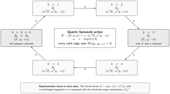
The quartic covariance orbit. Every edge carries adjacent canonical lines with $\Wr[y_k,y_{k+1}]=2\ii$. The pair $(E,g)$ returns after three steps, but $\alpha$ changes sign; all parameters and the sector label return only after six. The representative then carries formal holonomy, and an added inverse-square term also contributes local monodromy at the origin.

For example, the general Stokes-coefficient law gives

$$\begin{aligned} C_1(E,g,\alpha) &= \omega^{-\alpha} C_0(\omega^2E,\omega^4g,-\alpha), \\ C_2(E,g,\alpha) &= \omega^{2\alpha} C_0(\omega^4E,\omega^2g,\alpha). \end{aligned}$$

After six steps the canonical representative satisfies

$$y_{k+6} = -\ee^{-\pi\ii(-1)^k\alpha}y_k.$$

At $\alpha=0$ this becomes the homogeneous return $y_{k+6}=-y_k$.

A zero-energy audit

Set $g=\alpha=E=0$. The positive-sector quartic solution is elementary in terms of a modified Bessel function:

$$y_0(x,0) = \sqrt{\frac{2x}{3\pi}} K_{1/6}\!\left(\frac{x^3}{3}\right).$$

The large-argument expansion of $K_{1/6}$ gives exactly $x^{-1}\ee^{-x^3/3}$, so the leading coefficient agrees with the page’s canonical convention. Write

$$A=y_0(0,0), \qquad B=y_0'(0,0).$$

The small-argument expansion of $K_{1/6}$ yields

$$AB=-2.$$

Since

$$\begin{aligned} y_k(0,0)&=\omega^{k/2}A, & y_k'(0,0)&=\omega^{-k/2}B, \end{aligned}$$

one finds independently

$$\begin{aligned} \Wr[y_k,y_{k+1}](0) &=2\ii, \\ \Wr[y_{-1},y_1](0) &=2\ii\sqrt3, \\ C_0(0) &=\sqrt3. \end{aligned}$$

This exact value checks the half-power convention, the sign of the Wronskian, and the normalization of the scalar Stokes coefficient at once.

The harmonic threshold moves the phase into the energy

The assumption $M>1$ was structural, not cosmetic. For the harmonic oscillator,

$$\sqrt{x^2-E} = x-\frac{E}{2x}+O(x^{-3}),$$

so

$$b(E)=-\frac{E}{2}.$$

With $\omega=\ii$ the globally adjacent-normalized orbit is therefore

$$y_k(x,E) = \omega^{k/2+k(-1)^kE/2} y_0(\omega^{-k}x,(-1)^kE).$$

It still has $\Wr[y_k,y_{k+1}]=2\ii$, but its four-step return is

$$y_{k+4} = -\ee^{\pi\ii(-1)^kE}y_k.$$

The family-covariant convention often printed in the literature is

$$Y_k = \omega^{k/2-kE/2} y_0(\omega^{-k}x,(-1)^kE).$$

It agrees with the global gauge for $k=-1,0,1$, but farther around the orbit

$$\begin{aligned} \Wr[Y_k,Y_{k+1}] &= 2\ii\,\omega^{-E[k+(1-s_k)/2]}, \\ Y_{k+4} &= -\ee^{-\pi\ii E}Y_k. \end{aligned}$$

A third, naive convention retains only the factor $\omega^{k/2}$. Its first adjacent Wronskian is

$$\Wr[y_0,y_1] = 2\ii\ee^{\pi\ii E/4}.$$

All three gauges describe the same recessive lines. They place the same zero-free exponential in different connection coefficients. This is the same order-one normalization freedom exposed by the reciprocal-gamma determinants on Page 1.

Common pitfalls

Rotating only the spectral parameter. A lower monomial $g_ax^a$ has weight $a+2$. Unless its coupling is zero or fixed by that phase, the rotated energy belongs to a different point of the parameter family.

Normalizing only the recessive line. Recession fixes a one-dimensional line, not an absolute representative. Omitting the logarithmic WKB phase preserves spectral zeros but changes Wronskians, Stokes coefficients, and formal return factors.

Confusing sector closure with representative periodicity. After $2M+2$ steps the projected decay sector and polynomial passport return. The normalized solution may still acquire formal holonomy, and a singular finite point may act by a non-scalar monodromy matrix.

Importing the polynomial return to a branched potential. For $2M\notin\mathbb Z$, sectors live on a declared cover. A root-of-unity closure exists only when the covering and formal normalization actually support it.

Exercises

1. Derive every coupling weight. Starting from $x=\omega^kX$, prove

$$E\mapsto\omega^{2k}E, \qquad g_a\mapsto\omega^{(a+2)k}g_a.$$

Why may a constant term be absorbed into $E$?

Solution

The derivative contributes $\omega^{-2k}$ and $x^a=\omega^{ak}X^a$. Multiplying the equation by $\omega^{2k}$ therefore gives the coefficient $\omega^{(a+2)k}g_a$ and energy $\omega^{2k}E$. The constant term appears only through $g_0-E$, and both entries have the same weight.

2. Find the logarithmic WKB term. For $P=x^{2M}+\alpha x^{M-1}$ with $M>1$, expand $\sqrt{P-E}$ far enough to determine $b$ and the algebraic power of the recessive solution.

Solution

Factor out $x^{2M}$:

$$\begin{aligned} \sqrt{P-E} &= x^M\left( 1+\alpha x^{-M-1}-Ex^{-2M} \right)^{1/2} \\ &= x^M+\frac{\alpha}{2x}+O(x^{-M}). \end{aligned}$$

Thus $b=\alpha/2$. Integration contributes $(\alpha/2)\log x$, while the WKB amplitude contributes $x^{-M/2}$. The recessive solution therefore has the power $x^{-M/2-\alpha/2}$.

3. Check the global adjacent gauge. Use the displayed asymptotics to prove $\Wr[y_k,y_{k+1}]=2\ii$ for arbitrary $k$.

Solution

The two leading coefficients are $\ii^k$ and $\ii^{k+1}$. Their algebraic powers add to $-M$ because $s_{k+1}=-s_k$. The leading derivatives have signs $-s_k$ and $s_k$, so

$$\begin{aligned} \Wr[y_k,y_{k+1}] &= 2s_k\ii^k\ii^{k+1} \\ &= 2(-1)^k(-1)^k\ii =2\ii. \end{aligned}$$

The Wronskian is independent of $x$, so its asymptotic value is exact.

4. Recover the shifted-Wronskian phase. Derive the rotation law for $W_{j+r,k+r}$, accounting explicitly for the derivative Jacobian. Why is there no logarithmic phase for adjacent indices?

Solution

Each shifted solution contributes $\omega^{r/2-rs_{\bullet+r}b}$, while differentiating with respect to $x$ contributes $\omega^{-r}$. Multiplication gives

$$\omega^{-rb(s_{j+r}+s_{k+r})}.$$

For $k=j+1$, the two signs are opposite and their sum vanishes.

5. Complete the quartic passport. List $\mathcal R_k(E,g,\alpha)$ for $k=0,\ldots,6$. Identify the smallest positive returns of $(E,g)$, of $\alpha$, and of the full passport.

Solution

With $\zeta=\omega^2$,

$$\begin{array}{c|c} k&\mathcal R_k(E,g,\alpha)\\ \hline 0&(E,g,\alpha)\\ 1&(\zeta E,\zeta^2g,-\alpha)\\ 2&(\zeta^2E,\zeta g,\alpha)\\ 3&(E,g,-\alpha)\\ 4&(\zeta E,\zeta^2g,\alpha)\\ 5&(\zeta^2E,\zeta g,-\alpha)\\ 6&(E,g,\alpha) \end{array}$$

The pair $(E,g)$ returns after three steps, $\alpha$ after two, and the full passport after $\operatorname{lcm}(2,3)=6$.

6. Derive the quartic scalar phases. Starting from the general formula for $C_k$, obtain $C_1$ and $C_2$ for the quartic family.

Solution

Here $b=\alpha/2$. For $k=1$, $s_1=-1$, so the prefactor is $\omega^{-\alpha}$ and the passport is $(\omega^2E,\omega^4g,-\alpha)$. For $k=2$, $s_2=1$, so the prefactor is $\omega^{2\alpha}$ and the passport is $(\omega^4E,\omega^8g,\alpha)=(\omega^4E,\omega^2g,\alpha)$.

7. Audit the zero-energy quartic multiplier. Use $AB=-2$ and the endpoint rotation formulas to compute $W_{0,1}(0)$ and $W_{-1,1}(0)$.

Solution

At $M=2$, $\omega=\ee^{\pi\ii/3}$. Hence

$$\begin{aligned} W_{0,1}(0) &= AB(\omega^{-1/2}-\omega^{1/2}) =2\ii, \\ W_{-1,1}(0) &= AB(\omega^{-1}-\omega) =2\ii\sqrt3. \end{aligned}$$

Division by $2\ii$ gives $C_0(0)=\sqrt3$.

8. Separate two kinds of return. Suppose an inverse-square term is present and $2l+1\notin\mathbb Z$. Explain why returning to the same decay sector does not generally make $y_{k+N}$ proportional to $y_k$ by the formal phase alone.

Solution

The two local Frobenius lines at the origin have monodromy eigenvalues $\ee^{2\pi\ii(l+1)}$ and $\ee^{-2\pi\ii l}$. A solution selected by recession at infinity is generally a nontrivial linear combination of both. A complete turn therefore acts on it by the local monodromy matrix, not by one scalar eigenvalue. The formal phase at infinity must be multiplied by this finite-point continuation.

References

• Y. Sibuya, Global Theory of a Second Order Linear Ordinary Differential Equation with a Polynomial Coefficient, North-Holland Mathematics Studies 18, 1975, for canonical solutions, coefficient rotations, Wronskians, and global continuation for polynomial equations.
• P. Dorey and R. Tateo, “On the Relation between Stokes Multipliers and the T–Q Systems of Conformal Field Theory”, Nuclear Physics B 563 (1999), 573–602, with erratum, for the normalized homogeneous Symanzik family, adjacent Wronskians, finite return, the exact zero-energy Bessel normalization, and the harmonic-oscillator modification.
• P. Dorey, C. Dunning, and R. Tateo, “Spectral Equivalences, Bethe Ansatz Equations, and Reality Properties in PT-Symmetric Quantum Mechanics”, Journal of Physics A 34 (2001), 5679–5704, especially Section 2 for the primary normalized treatment of $x^{2M}+\alpha x^{M-1}+l(l+1)/x^2$, the alternating sign of $\alpha$, and the coupled central Stokes relations.
• P. Dorey, C. Dunning, and R. Tateo, “The ODE/IM Correspondence”, Journal of Physics A 40 (2007), R205–R283, especially Sections 4.2, 5.3, and 6.1 and Appendix B for the homogeneous rotation, finite-cover return, the $\alpha$ deformation, and the harmonic threshold.
• K. C. Shin, “Eigenvalues of PT-Symmetric Oscillators with Polynomial Potentials”, Journal of Physics A 38 (2005), 6147–6166, for canonical polynomial solutions, the raw coefficient rotations, and Wronskian covariance retaining the logarithmic WKB coefficient. The extra rephasing that makes all adjacent Wronskians $2\ii$ is derived on this page.
• E. Delabaere and J.-M. Rasoamanana, “Resurgent Deformations for an Ordinary Differential Equation of Order 2”, Pacific Journal of Mathematics 223 (2006), 35–93, for a rigorous treatment of polynomial-over-$x^2$ equations, canonical solutions, and the interaction between infinity data and finite-origin monodromy.
• H. E. Gollwitzer and Y. Sibuya, “Stokes Multipliers for Subdominant Solutions of Second Order Differential Equations with Polynomial Coefficients”, Journal für die reine und angewandte Mathematik 243 (1970), 98–119, for the primary global construction of scalar Stokes multipliers for polynomial coefficients.
• NIST Digital Library of Mathematical Functions, §10.25 on modified Bessel functions and §10.30 on limiting forms, for the exact zero-energy quartic audit.