ODE/IM TBA from TQ and Y-System Analyticity

Chapter 12 ended with exact functional relations and a warning: algebra does not choose an analytic solution. A $TQ$ equation knows how shifted functions fit together, and a $Y$-system knows a finite-difference operator, but neither specifies which logarithm to take, which zeros a contour encloses, which asymptotic solution is physical, or which homogeneous term survives Fourier inversion.

Those are precisely the data that turn a functional relation into a nonlinear integral equation. The central principle of this chapter is therefore:

The analytic contract

A $Y$-system supplies the difference operator. Analyticity, nonvanishing, asymptotics, and contour data select its inverse and therefore the state.

This page states that contract, keeps the TQ and fused-$Y$ routes separate, and proves one scalar calibration completely. The detailed strip lemmas, matrix kernels, driving-term calculations, source terms, and numerical algorithms belong to the pages that follow.

Chapter question

How are ODE/IM functional relations converted into nonlinear integral equations and exact numerical data, and which analytic hypotheses make that conversion reversible?

Status ledger

Passage	Status on this page
Chapter 12 $TQ$, fusion, and $Y$ identities	Exact in the ODE and model passports already declared there
Multiplicative shift $s\mapsto q^js$ to an additive rapidity shift	Exact on a chosen logarithmic cover
Multiplicative relation to an equation for logarithms	Conditional on nonvanishing, boundary values, and a fixed branch integer
Removal of the growing asymptotic	Model-dependent input from ODE/WKB or integrable-model asymptotics
Scalar convolution formula below	A theorem under its stated strip and integrability hypotheses
Ground-state or excited-state interpretation	Requires a zero, contour, reality, and state passport
Equality with an exact-WKB/GMN integral equation	Not asserted; Pages 3 and 4 treat that separate question

Three integral-equation languages have different unknowns

The phrases “TBA equation” and “NLIE” are often used too loosely. Three constructions occur in this book, and a formula from one cannot be moved to another merely because all three contain logarithms and convolutions.

Route	Primary unknown	Discrete data	What closes the derivation
TQ/Destri–de Vega	Auxiliary ratio $a$ or a counting function	Zeros of $1+a$, separated into roots, holes, and transfer zeros	A contour around the intended divisor, plus large-rapidity data
Fused $Y$-system TBA	Node functions $Y_a$ or pseudoenergies $\varepsilon_a$	Zeros and poles of $Y_a$ and $1+Y_a$	A finite fusion graph, analytic strips, branches, and a matrix inverse
Exact-WKB/GMN Riemann–Hilbert equation	Resummed periods or Darboux coordinates	BPS charges, intersection pairings, and Stokes rays	A Riemann–Hilbert jump problem and its asymptotic normalization

The first two are ODE/IM inversion routes. The third starts from exact-WKB jump data and will enter on Page 3. Any equivalence between them is an additional theorem for a specified example, not a generic identity.

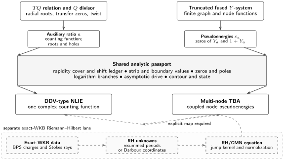
The three inversion routes use different unknowns and different discrete data. The two ODE/IM lanes share an analytic passport but not necessarily the same kernel or contour. The exact-WKB lane is separate until an explicit map of variables, jumps, asymptotics, and normalizations is proved.

A rapidity coordinate turns rotations into translations

Retain the Chapter 12 homogeneous-oscillator conventions

$$q=\exp\!\left(\frac{\pi\ii}{M+1}\right), \qquad \rho_M=\frac{M+1}{2M}.$$

Choose a positive scale $s_\star$ and the growth-adapted logarithmic coordinate

$$\theta =\rho_M\Log\!\left(\frac{s}{s_\star}\right), \qquad s=s_\star \exp\!\left(\frac{2M}{M+1}\theta\right).$$

The logarithm is part of the parameter passport. On this cover,

$$\begin{aligned} q^{\pm1}s &\longleftrightarrow \theta\pm\frac{\pi\ii}{2M}, \\ q^{\pm2}s &\longleftrightarrow \theta\pm\frac{\pi\ii}{M}. \end{aligned}$$

This is why the shift ledger from Chapter 12 matters: fusion relations use $q^{\pm1}s$, while the elementary Baxter equation and the auxiliary root ratios use $q^{\pm2}s$. The two additive shifts differ by a factor of two.

The same coordinate also linearizes the leading growth. Since a homogeneous determinant has

$$\log D(s)\sim c\,s^{\rho_M},$$

its rapidity asymptotic is proportional to $e^\theta$. The coordinate has therefore matched two independent structures: the rotation angle and the WKB growth order.

For the particularly simple polynomial closure used here, take $l=0$ and integer $M>1$, and put

$$h=2M.$$

The finite $A_{h-1}$ system of Chapter 12 then has the standard shift $\theta\mapsto\theta\pm\pi\ii/h$. For the quartic oscillator, $M=2$ and $h=4$: a $q$-shift is $\pm\pi\ii/4$, while a $q^2$-shift is $\pm\pi\ii/2$.

The TQ and fused-Y routes carry different divisor ledgers

The TQ route begins from the Page 6 auxiliary functions

$$\begin{aligned} a_+(s) &=\ee^{2\ii\vartheta} \frac{Q_+(q^2s)}{Q_+(q^{-2}s)}, \\ a_-(s) &=\ee^{-2\ii\vartheta} \frac{Q_-(q^2s)}{Q_-(q^{-2}s)}. \end{aligned}$$

Their factorized TQ equations imply

$$1+a_\pm(s) =\ee^{\pm\ii\vartheta} \frac{T(s)Q_\pm(s)}{Q_\pm(q^{-2}s)}.$$

Thus $1+a_\pm=0$ does not label one spectrum by itself. Subject to the displayed denominator, it can detect a radial determinant zero, a transfer-function zero, or—after a contour has been deformed—a hole.

A useful model-specific separation theorem is available for the regular radial oscillator when

$$M>1, \qquad -\frac12<l<\frac M2.$$

In this window the radial $Q_+$ zeros are positive and simple, while the associated lateral-transfer zeros are negative. A contour around the positive ray can therefore select exactly the radial divisor. This is spectral input from self-adjointness and the PT-symmetric lateral problem—not a consequence of the $TQ$ identity—and Page 2 will state the contour formula in that passport.

The DDV-type route replaces the logarithmic derivative of a product over the selected roots by a Cauchy integral of $\log(1+a)$. Its characteristic shape is

$$\begin{aligned} \log a ={}&\text{twist}+\text{driving term} \\ &+\text{one boundary-value convolution} \\ &-\text{the opposite boundary-value convolution} \\ &+\text{declared source terms}. \end{aligned}$$

This line is structural, not a contour formula. The contour orientation, kernel, boundary values, and sources are model data and will be derived on Page 2.

The fused route starts instead from the finite nearest-neighbor system

$$\begin{aligned} &Y_a\!\left(\theta+\frac{\pi\ii}{h}\right) Y_a\!\left(\theta-\frac{\pi\ii}{h}\right) \\ &\qquad= \prod_{b=1}^{h-1} \bigl(1+Y_b(\theta)\bigr)^{I_{ab}}, \qquad a=1,\ldots,h-1, \end{aligned}$$

where $I$ is the $A_{h-1}$ incidence matrix. This route exists as a finite TBA only when the fusion orbit actually truncates. For generic $M$ the one-function TQ/NLIE route may still exist even though no finite $Y$-graph closes.

Explicitly,

$$I_{ab}=\delta_{a,b+1}+\delta_{a,b-1}, \qquad Y_0=Y_h=0.$$

Logarithms create a strip boundary-value problem

Assume first that the ground-state $Y_a$ are positive on the real line and that both $Y_a$ and $1+Y_a$ are nonzero on a simply connected domain containing the shifted contours. Equivalently, one may assume directly that the required single-valued logarithms have been chosen with zero winding. Define the Dorey–Dunning–Tateo pseudoenergy convention

$$\varepsilon_a=\Log Y_a, \qquad L_a=\log\!\left(1+\ee^{-\varepsilon_a}\right).$$

Because

$$\log(1+Y_b)=\varepsilon_b+L_b,$$

the multiplicative system becomes

$$\begin{aligned} &\varepsilon_a\!\left(\theta+\frac{\pi\ii}{h}\right) +\varepsilon_a\!\left(\theta-\frac{\pi\ii}{h}\right) -\sum_b I_{ab}\varepsilon_b(\theta) \\ &\qquad= \sum_b I_{ab}L_b(\theta)+2\pi\ii N_a. \end{aligned}$$

The integer $N_a$ is not decorative. On a connected region where all logarithm arguments are nonzero and the branches vary continuously, it is locally constant. A zero or pole of $Y_a$, a zero of $1+Y_a$, or a crossed cut can change the branch ledger and introduce a source.

The leading ODE asymptotic supplies a homogeneous solution

$$d_a(\theta) =\kappa\sin\!\left(\frac{\pi a}{h}\right)\ee^\theta.$$

Indeed, the sine vector is the Perron–Frobenius eigenvector of the incidence matrix:

$$\sum_b I_{ab}\sin\!\left(\frac{\pi b}{h}\right) =2\cos\!\left(\frac{\pi}{h}\right) \sin\!\left(\frac{\pi a}{h}\right),$$

while shifting $e^\theta$ by $\pm\pi\ii/h$ produces the same factor. Thus the difference equation cannot determine the coefficient $\kappa$. That coefficient is fixed by determinant/WKB asymptotics and is part of the state passport.

For the ground-state branch considered here, choose the continuous logarithms with $N_a=0$. A nonzero $N_a$ would contribute at zero Fourier momentum and must be retained as a constant particular solution or an explicit source.

There is one more endpoint issue. In the finite ODE system, $f_a=\varepsilon_a-d_a$ and $L_a$ generally approach nonzero zero-spectral constants as $\theta\to-\infty$. Their Fourier transforms are therefore not ordinary $L^1$ transforms. After a boundary regulator or an equivalent distributional prescription has been declared, the nonzero-momentum multiplier to invert is

$$\begin{aligned} \sum_b \mathcal A_{ab}(k)\widehat f_b(k) &= \sum_b I_{ab}\widehat L_b(k), \qquad k\ne0, \\ \mathcal A_{ab}(k) &= 2\cosh\!\left(\frac{\pi k}{h}\right)\delta_{ab}-I_{ab}. \end{aligned}$$

Inverting this matrix produces the nonzero-momentum part of the multi-node TBA kernel. This compact formula records the algebraic step; Page 2 will restore the regulated endpoint constants and justify the contour shifts, invertibility, and real-space kernels.

ANZC belongs to the normalized remainder

The common shorthand ANZC means analytic, nonzero, and constant-asymptotic in a declared strip. It is rarely the raw pseudoenergy that has this property. In the finite fused system, $\varepsilon_a\sim d_a$ as $\Re\theta\to+\infty$, so the useful object is

$$\exp\!\left(\varepsilon_a-d_a\right) =\ee^{-d_a}Y_a.$$

In the scalar convention used below, $Y=\ee^{-\varepsilon}$ tends to zero and the stripped object is instead $\ee^dY$. The sign changes with the pseudoenergy convention; the principle does not.

A sufficient inversion passport records all of the following:

1. the logarithmic cover and the exact strip width;
2. analyticity and nonvanishing of every logarithm argument;
3. controlled boundary values on both shifted lines;
4. the branch integers and Schwarz-reflection convention;
5. the complete growing asymptotic to subtract;
6. integrability or Hardy-class control of the remainder;
7. the zeros, poles, holes, and contour indentations assigned to the chosen state.

Checking only the real axis is not enough. Nor does the entirety of a function in $s$ prove nonvanishing after the exponential pullback to a rapidity strip.

A scalar zero-free strip yields a prototype TBA equation

The matrix system above is the actual finite ODE/IM route. To calibrate the analytic inversion without graph notation, consider the one-component prototype

$$Y(u+\ii\eta)Y(u-\ii\eta)=1+Y(u), \qquad Y=\ee^{-\epsilon}.$$

This is a normalization model, not the physical quartic-oscillator TBA, which has the $A_3$ graph. Assume:

• $\eta>0$ and $R>0$;
• $Y$ and $1+Y$ are analytic and nonzero for $|\Im u|<\eta$ and have controlled boundary values;
• $Y(\bar u)=\overline{Y(u)}$ and $Y(u)>0$ for real $u$;
• the continuous logarithms are chosen with branch integer $N=0$;
• with $$d(u)=R\cosh\!\left(\frac{\pi u}{2\eta}\right),$$ the remainder $v=\epsilon-d$ is analytic in the strip, has $L^1$ boundary values, and obeys the Hardy-type bound $$\sup_{|y|<\eta} \int_{\mathbb R}|v(x+\ii y)|\,\dd x<\infty;$$
• $L=\log(1+\ee^{-\epsilon})$ belongs to $L^1(\mathbb R)$, and the vertical-edge integrals vanish in the boundary contour shifts.

The logarithmic equation is

$$\epsilon(u+\ii\eta)+\epsilon(u-\ii\eta)=-L(u).$$

The driving term is invisible because

$$d(u+\ii\eta)+d(u-\ii\eta)=0.$$

Therefore $v^++v^-=-L$. Fix the Fourier convention

$$\begin{aligned} \widehat f(k) &=\int_{\mathbb R}\ee^{\ii ku}f(u)\,\dd u, \\ f(u) &=\frac{1}{2\pi} \int_{\mathbb R}\ee^{-\ii ku}\widehat f(k)\,\dd k. \end{aligned}$$

Analytic contour shifts give

$$\widehat{v(\,\cdot+\ii\eta\,)}(k) =\ee^{\eta k}\widehat v(k), \qquad \widehat{v(\,\cdot-\ii\eta\,)}(k) =\ee^{-\eta k}\widehat v(k).$$

Hence

$$2\cosh(\eta k)\widehat v(k)=-\widehat L(k).$$

With $(K*f)(u)=\int_{\mathbb R}K(u-u')f(u')\,\dd u'$, the inverse kernel is

$$\begin{aligned} \widehat K_\eta(k) &=\frac{1}{2\cosh(\eta k)}, \\ K_\eta(u) &=\frac{1}{4\eta} \operatorname{sech}\!\left(\frac{\pi u}{2\eta}\right). \end{aligned}$$

The prototype TBA equation is therefore

$$\begin{aligned} \epsilon(u) ={}&R\cosh\!\left(\frac{\pi u}{2\eta}\right) \\ &- \int_{\mathbb R} K_\eta(u-u') \log\!\left(1+\ee^{-\epsilon(u')}\right) \,\dd u'. \end{aligned}$$

At the standard calibration $\eta=\pi/2$,

$$\begin{aligned} \epsilon(u) ={}&R\cosh u \\ &- \int_{-\infty}^{\infty} \frac{\log\!\left(1+\ee^{-\epsilon(u')}\right)} {2\pi\cosh(u-u')} \,\dd u'. \end{aligned}$$

Two normalization checks are immediate. First,

$$\int_{\mathbb R}K_\eta(u)\,\dd u =\widehat K_\eta(0)=\frac12,$$

The zero-drive case $R=0$ lies outside the $L^1$ hypotheses used in the Fourier derivation. The same equation nevertheless has a bounded-convolution extension because $K_\eta\in L^1$. In that extension, the positive constant solution is

$$Y=\frac{1+\sqrt5}{2}.$$

Indeed $Y^2=1+Y$, while the integral equation gives $-\log Y=-\tfrac12\log(1+Y)$. The two calculations agree only with the kernel normalization shown above.

For this real scalar calibration with $R\geq0$, the fixed-point map for the bounded remainder is a contraction because $|\dd\log(1+\ee^{-x})/\dd x|\le1$ and $\lVert K_\eta\rVert_1=1/2$. This proves uniqueness in the toy class. It does not prove uniqueness for complex twists, matrix systems, excited-state contours, or kernels after analytic continuation.

What the integral equation determines

Solving an NLIE or TBA determines the analytic function named in its passport on the integration contour. Recovering ODE spectral data then requires the declared dictionary back to $T$, $Q$, or a determinant, analytic continuation to the quantization locus, and one absolute normalization or WKB asymptotic.

For a TQ auxiliary ratio, simple roots obey

$$a(\theta_j)=-1, \qquad \Log a(\theta_j)=\pi\ii(2I_j+1),$$

where the integers $I_j$ are branch and quantum-number data. The ratio form additionally assumes that the shifted denominator is nonzero. If both shifted $Q$-values vanish, one must return to the denominator-free TQ equation.

A solved $Y$-system TBA can similarly reconstruct selected transfer or determinant combinations, but not the full ODE connection matrix. It also does not retroactively prove the zero locations or strip nonvanishing assumed in its derivation.

The rest of Chapter 13 supplies the missing layers: Page 2 proves the strip, kernel, driving, and contour machinery; Pages 3 and 4 introduce the exact-WKB/GMN construction and audit possible equivalences; Page 5 adds excited-state sources and wall crossing; Page 6 treats numerical convergence and error; Page 7 compares WKB and NS periods; and Page 8 performs a full spectral computation.

Common pitfalls

Taking logarithms after checking only $Y$. The argument $1+Y$ must also be nonzero on the chosen domain. Its zeros are precisely where a new logarithmic source can enter.

Using the same rapidity shift for $q$ and $q^2$. In the convention above they give $\pi\ii/(2M)$ and $\pi\ii/M$. Confusing them changes the Fourier multiplier and the kernel.

Fourier transforming the growing pseudoenergy. The driving term is not integrable. Subtract it first and transform only the controlled remainder.

Deriving the drive from the $Y$-system. The drive is a homogeneous mode invisible to the difference equation. ODE/WKB asymptotics fix its coefficient.

Calling every nonlinear equation TBA. A DDV counting-function NLIE, a fused-node TBA, and a GMN Riemann–Hilbert equation have different unknowns and divisor data.

Inferring a strip from a real-axis plot. A numerical scan can miss a nearby complex zero or pole. The contour shift needs control on the whole strip and its boundary values.

Promoting one convergent iteration to uniqueness. The scalar toy model has a contraction proof. General ODE/IM equations require their own existence and uniqueness analysis.

Exercises

1. Audit the multiplicative-to-additive shift

Starting from

$$q=\exp\!\left(\frac{\pi\ii}{M+1}\right), \qquad \theta=\frac{M+1}{2M}\Log\!\left(\frac{s}{s_\star}\right),$$

derive the rapidity displacement produced by $s\mapsto q^js$. Then specialize to the $q$- and $q^2$-shifts for the quartic oscillator.

Solution

On the chosen logarithmic sheet,

$$\Log\!\left(\frac{q^js}{s_\star}\right) =\Log\!\left(\frac{s}{s_\star}\right) +\frac{j\pi\ii}{M+1}.$$

Multiplication by $(M+1)/(2M)$ gives

$$s\mapsto q^js \quad\Longleftrightarrow\quad \theta\mapsto\theta+\frac{j\pi\ii}{2M}.$$

For $M=2$, a $q$-shift gives $\pi\ii/4$ and a $q^2$-shift gives $\pi\ii/2$. These are respectively the fusion and elementary TQ shifts in the conventions of this chapter.

2. Prove that the logarithmic defect is locally constant

Suppose all factors in a multiplicative $Y$-system are nonzero on a connected domain $U$, and continuous logarithms have been selected. Show that the discrepancy between the two logarithmic sides is $2\pi\ii N$ with $N$ locally constant. State how $N$ can change.

Solution

Let $F$ be the logarithm of the left-hand side minus the logarithm of the right-hand side. The multiplicative identity implies

$$\ee^{F(u)}=1.$$

Consequently $F(u)/(2\pi\ii)$ is integer-valued. It is also continuous on $U$, because every chosen logarithm is continuous there. A continuous integer-valued function on a connected set is constant, so $F=2\pi\ii N$ for one integer $N$ on each connected component.

The argument fails when a factor $Y_a$ or $1+Y_a$ vanishes or has a pole, when a shifted contour crosses a cut, or when the domain is split. Crossing such an obstruction can change $N$ and can also generate an explicit source term.

3. Separate what ANZC does and does not prove

Let $d$ and $g$ be analytic in a strip, with $g$ non-singular there and $g(u)\to0$ at both asymptotic ends. Set

$$Y(u)=\ee^{d(u)+g(u)}.$$

Which ANZC properties follow for $\ee^{-d}Y$? Does this information alone justify taking $\Log(1+Y)$ and shifting its contour?

Solution

The stripped function is

$$\ee^{-d(u)}Y(u)=\ee^{g(u)}.$$

It is analytic and nonzero wherever $g$ is analytic, and it tends to $1$ at both stated ends. Thus it has the advertised analytic, nonzero, constant-asymptotic behavior in the open strip.

This does not imply that $1+Y$ is nonzero: the value $Y=-1$ is compatible with $Y\ne0$. Nor does open-strip analyticity by itself give the boundary estimates needed to move a Fourier contour. One must check $1+Y$, boundary values, branch continuity, and suitable decay or Hardy-class control separately.

4. Verify the invisible ODE driving mode

For the $A_{h-1}$ incidence matrix, show that

$$d_a(\theta) =\kappa\sin\!\left(\frac{\pi a}{h}\right)\ee^\theta$$

solves the homogeneous logarithmic $Y$-system operator.

Solution

With the boundary convention $d_0=d_h=0$, the incidence matrix gives

$$\begin{aligned} \sum_b I_{ab}d_b(\theta) &=d_{a-1}(\theta)+d_{a+1}(\theta) \\ &=2\cos\!\left(\frac{\pi}{h}\right)d_a(\theta). \end{aligned}$$

On the other hand,

$$\begin{aligned} d_a\!\left(\theta+\frac{\pi\ii}{h}\right) +d_a\!\left(\theta-\frac{\pi\ii}{h}\right) &=\left(\ee^{\pi\ii/h}+\ee^{-\pi\ii/h}\right)d_a(\theta) \\ &=2\cos\!\left(\frac{\pi}{h}\right)d_a(\theta). \end{aligned}$$

Their difference is zero. Hence the functional relation cannot fix $\kappa$; the ODE/WKB asymptotic must do so.

5. Reconstruct the scalar inversion kernel

Using the Fourier convention on this page, derive the multiplier and real-space kernel that invert

$$v(u+\ii\eta)+v(u-\ii\eta)=-L(u).$$

Check the total mass of the kernel.

Solution

Analytic contour displacement gives

$$\widehat{v(\,\cdot+\ii\eta\,)} =\ee^{\eta k}\widehat v(k), \qquad \widehat{v(\,\cdot-\ii\eta\,)} =\ee^{-\eta k}\widehat v(k).$$

Therefore

$$\widehat v(k) =-\frac{\widehat L(k)}{2\cosh(\eta k)}.$$

The standard transform pair yields

$$\widehat K_\eta(k)=\frac{1}{2\cosh(\eta k)}, \qquad K_\eta(u)=\frac{1}{4\eta} \operatorname{sech}\!\left(\frac{\pi u}{2\eta}\right).$$

Thus $v=-K_\eta*L$. Evaluating the multiplier at zero, or integrating the hyperbolic secant directly, gives

$$\int_{\mathbb R}K_\eta(u)\,\dd u =\widehat K_\eta(0)=\frac12.$$

6. Audit the TQ divisor before drawing a contour

Use

$$1+a_\pm(s) =\ee^{\pm\ii\vartheta} \frac{T(s)Q_\pm(s)}{Q_\pm(q^{-2}s)}$$

to classify a zero of $1+a_\pm$. What can be concluded when the zero comes from $Q_\pm$, from $T$, or at a point where the shifted denominator vanishes? Where do holes enter this ledger?

Solution

Assume first that $Q_\pm(q^{-2}s_\star)\ne0$. If $Q_\pm(s_\star)=0$ and $T(s_\star)\ne0$, then $s_\star$ is a radial determinant zero. If $T(s_\star)=0$ and $Q_\pm(s_\star)\ne0$, it is a lateral or transfer-function zero. If both numerator factors vanish, the equation alone does not assign the zero to one spectral problem; the declared divisors and multiplicities must be inspected.

A hole is not a third factor in the displayed identity. It is a state-and-contour label for a solution of $1+a=0$ that is not occupied by the selected $Q$-root set; in the ODE factorization it is typically tracked through the transfer divisor after a contour deformation.

If $Q_\pm(q^{-2}s_\star)=0$, the ratio defining $a_\pm$ is singular or indeterminate, so the factorized equation is not a safe quantization test. One must return to the denominator-free TQ relation and test for cancellation before assigning any spectral meaning.

7. Check the quartic zero-spectral A₃ solution

The quartic fusion values at zero spectral parameter are

$$(T_0,T_{1/2},T_1,T_{3/2},T_2,T_{5/2}) (0)=(1,\sqrt3,2,\sqrt3,1,0).$$

Using

$$Y_n=T_{(n-1)/2}T_{(n+1)/2},$$

compute $(Y_1,Y_2,Y_3)$ and verify the constant $A_3$ $Y$-system.

Solution

The three node values are

$$(Y_1,Y_2,Y_3)=(2,3,2).$$

With $Y_0=Y_4=0$, the constant nearest-neighbor equations are

$$Y_a^2=(1+Y_{a-1})(1+Y_{a+1}).$$

For the end nodes, $2^2=(1+0)(1+3)=4$. For the middle node, $3^2=(1+2)(1+2)=9$. This also shows why the scalar golden-ratio calibration is not the quartic oscillator: the latter has three coupled nodes and different constant data.

8. Audit a claimed equivalence of nonlinear equations

Two authors begin from the same multiplicative $Y$-system but obtain integral equations with different driving terms. Explain why the common functional relation does not prove that the equations are equivalent. Give a minimal comparison checklist.

Solution

The linear difference operator cannot determine a homogeneous drive $d_a$, so an inversion must import its coefficient from asymptotics. This is not an additive symmetry of the nonlinear equation: although $\mathcal D H=0$, one generally has

$$\log\!\left(1+\ee^{-\varepsilon_a-H_a}\right) \ne \log\!\left(1+\ee^{-\varepsilon_a}\right).$$

Thus adding $H$ to a known solution need not produce another solution. Different driving asymptotics define different nonlinear boundary-value problems, and each candidate integral equation must be checked against the functional relation independently. The scalar family $d_R=R\cosh(\pi u/(2\eta))$ is the prototype: every $d_R$ is homogeneous, but the value of $R$ must be supplied before solving the fixed-point problem.

At minimum, one must match:

1. the unknown functions and rapidity variables;
2. the shift and Fourier conventions;
3. the analytic strip and its boundary values;
4. zeros, poles, holes, branch integers, and contour prescriptions;
5. the complete driving asymptotic and its normalization;
6. kernel normalizations and declared source terms;
7. the dictionary from the solution back to the same determinant or spectral observable.

Without these identifications, the two equations may be different inversions of the same algebraic relation rather than equivalent descriptions of the same state.

References

• Al. B. Zamolodchikov, “Thermodynamic Bethe Ansatz in Relativistic Models: Scaling Three-State Potts and Lee–Yang Models,” Nuclear Physics B 342 (1990), 695–720, doi:10.1016/0550-3213(90)90333-9. The foundational ground-state TBA construction and its scaling tests.
• V. V. Bazhanov, S. L. Lukyanov, and A. B. Zamolodchikov, “Integrable Structure of Conformal Field Theory, Quantum KdV Theory and Thermodynamic Bethe Ansatz,” Communications in Mathematical Physics 177 (1996), 381–398, arXiv:hep-th/9412229. The transfer-matrix functional relations and their ground-state TBA interpretation.
• V. V. Bazhanov, S. L. Lukyanov, and A. B. Zamolodchikov, “Integrable Structure of Conformal Field Theory II. Q-Operator and DDV Equation,” Communications in Mathematical Physics 190 (1997), 247–278, arXiv:hep-th/9604044, doi:10.1007/s002200050240. A primary derivation of a DDV equation from a Baxter relation under analytic assumptions.
• C. Destri and H. J. de Vega, “New Thermodynamic Bethe Ansatz Equations without Strings,” Physical Review Letters 69 (1992), 2313–2317, doi:10.1103/PhysRevLett.69.2313. The original one-function nonlinear-integral-equation framework.
• P. Dorey and R. Tateo, “Anharmonic Oscillators, the Thermodynamic Bethe Ansatz, and Nonlinear Integral Equations,” Journal of Physics A 32 (1999), L419–L425, arXiv:hep-th/9812211, doi:10.1088/0305-4470/32/38/102. The primary ODE/IM conversion from anharmonic-oscillator spectral determinants to a nonlinear integral equation.
• P. Dorey and R. Tateo, “On the Relation between Stokes Multipliers and the T–Q Systems of Conformal Field Theory,” Nuclear Physics B 563 (1999), 573–602, arXiv:hep-th/9906219, doi:10.1016/S0550-3213(99)00609-4, with erratum Nuclear Physics B 603 (2001), 581, doi:10.1016/S0550-3213(01)00163-8. The detailed ODE determinant, auxiliary-function, contour, and kernel conventions behind the DDV route.
• P. Dorey, C. Dunning, and R. Tateo, “Spectral Equivalences, Bethe Ansatz Equations, and Reality Properties in PT-Symmetric Quantum Mechanics,” Journal of Physics A 34 (2001), 5679–5704, arXiv:hep-th/0103051, doi:10.1088/0305-4470/34/28/305. The spectral-location result used to separate the radial and lateral divisors in the clean parameter window.
• P. Dorey, C. Dunning, and R. Tateo, “The ODE/IM Correspondence,” Journal of Physics A 40 (2007), R205–R283, arXiv:hep-th/0703066, doi:10.1088/1751-8113/40/32/R01. Section 6 and Appendices D–E give the fused-$Y$ and DDV routes with explicit analyticity assumptions and kernels.
• A. Kuniba, T. Nakanishi, and J. Suzuki, “T-Systems and Y-Systems in Integrable Systems,” Journal of Physics A 44 (2011), 103001, arXiv:1010.1344, doi:10.1088/1751-8113/44/10/103001. A broad reference for functional systems, analytic Bethe ansatz, and TBA inversion.