Stokes Multipliers and Rotated Spectral Problems

The preceding page used one solution recessive on the positive ray to construct two radial spectral determinants: the other end of the boundary problem was the regular point $x=0$. Polynomial infinity offers another possibility. A contour can begin in one decay sector at infinity and end in a different decay sector. The corresponding lateral boundary function is a Wronskian of two canonical recessive solutions.

That observation is the exact ODE core of this page. Three consecutive recessive lines give a scalar Stokes relation, and the scalar multiplying the middle solution is itself a nonadjacent Wronskian. Its zeros therefore select solutions that decay at both ends of a complex contour. Rotating the two ends produces a new spectral problem; rotating its energy requires an additional covariance of the entire ODE family.

The general existence theory and unipotent Stokes factors were developed in Chapter 1 and Chapter 2. Here they are specialized to a spectral family. The fully normalized Symanzik action belongs to Page 3, the Baxter identification to Page 4, and the $TQ$ and $Y$-system relations to Page 5.

The result to retain

Let $y_{k-1},y_k,y_{k+1}$ be canonically normalized solutions recessive in three consecutive sectors, with

$$\Wr[y_{k-1},y_k] = \Wr[y_k,y_{k+1}] = 2\ii.$$

Then

$$C_k(E)y_k = y_{k-1}+y_{k+1}, \qquad C_k(E) = \frac{\Wr[y_{k-1},y_{k+1}]}{2\ii}.$$

Thus $C_k(E)=0$ exactly when one nonzero solution is recessive in both nonadjacent sectors $\mathcal S_{k-1}$ and $\mathcal S_{k+1}$. This is a lateral spectral condition. No integrable model has been used.

Status ledger

Statement used on this page	Status
Existence of a unique canonically normalized recessive representative, entire in $E$ for fixed $x$	Classical global ODE theorem for the polynomial family and normalization stated below
Any two consecutive recessive solutions form a basis	Exact consequence of their opposite exponential behavior on a common asymptotic region
The raw three-solution and Wronskian identities	Exact two-dimensional linear algebra
A nonadjacent Wronskian zero means simultaneous recession at both contour ends	Exact boundary-line argument
Zeros of a nonzero entire boundary Wronskian are isolated	Exact complex analysis; identifying them as the discrete spectrum of a closed contour operator requires compact resolvent or an equivalent global boundary-value theorem
A shifted sector pair has a rotated zero set	Exact only when the coefficient family is rotation covariant and the contour is transformed with it
Equality of absolute Wronskian functions after rotation	Requires compatible canonical normalizations; a nowhere-zero factor is otherwise allowed
Reality of a PT-symmetric lateral spectrum	A separate spectral theorem under additional hypotheses, not a consequence of PT symmetry alone
A scalar Stokes multiplier is a transfer-matrix eigenvalue	Model-dependent ODE/IM dictionary, deferred

Polynomial infinity supplies a lifted family of recessive lines

Retain the homogeneous equation and normalization regime of Page 1,

$$\left[ -\frac{\dd^2}{\dd x^2}+x^{2M} \right]y(x,E) = E y(x,E), \qquad M\in\mathbb N, \quad M>1.$$

The restriction $M>1$ keeps the simple canonical form $x^{-M/2}\exp[-x^{M+1}/(M+1)]$ free of $E$-dependent logarithmic terms. At $M=1$, the spectral parameter enters the algebraic power and the recessive solution instead behaves as $x^{-1/2+E/2}\ee^{-x^2/2}$. This is also the threshold at which Page 1 found an order-one determinant, so the asymptotic-power and zero-free exponential conventions must be fixed together.

Set

$$N=2M+2$$

and define the open decay sectors

$$\mathcal S_k = \left\{ x: \left| \arg x-\frac{k\pi}{M+1} \right| < \frac{\pi}{2(M+1)} \right\}, \qquad k\in\mathbb Z.$$

The argument is initially lifted to the universal cover. Geometrically, $\mathcal S_{k+N}$ projects to the same wedge as $\mathcal S_k$, but an identification of the normalized solutions also involves their formal return. It should not be guessed from the picture alone.

In $\mathcal S_k$ the quantity $(-1)^kx^{M+1}$ has positive real part. There is a unique recessive line represented by a solution $\widehat y_k(x,E)$ with a fixed leading coefficient:

$$\widehat y_k(x,E) \sim A_k x^{-M/2} \exp\left[ -\frac{(-1)^k x^{M+1}}{M+1} \right].$$

The lift of $\arg x$, the branch of $x^{-M/2}$, and the nonzero coefficient $A_k$ are part of the normalization. For fixed $x$, the canonical solution and its derivative are entire in $E$. Changing $A_k$ by a nowhere-zero analytic factor preserves the recessive line and its spectral zeros but changes absolute connection coefficients.

Two neighboring solutions are independent. Continue both canonical solutions into a common proper subsector on which their enlarged Sibuya asymptotics hold. There one exponential is dominant precisely where the other is recessive. Hence

$$\Wr[\widehat y_k,\widehat y_{k+1}] \neq0,$$

and $(\widehat y_k,\widehat y_{k+1})$ is a basis of the two-dimensional solution space.

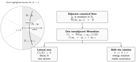
Sector and Wronskian geometry, shown for the quartic oscillator $M=2$. The radial problem joins $x=0$ to $\mathcal S_0$; the elementary lateral problem joins $\mathcal S_{-1}$ to $\mathcal S_1$. The algebraic relation among three canonical lines is exact. A shift of all sector labels rotates the boundary domain, while a corresponding energy rotation additionally uses covariance of the differential equation and its normalization.

Three sectors give one normalization-complete relation

Before choosing convenient constants, expand $\widehat y_{k-1}$ in the neighboring basis:

$$\widehat y_{k-1} = a_k\widehat y_k+b_k\widehat y_{k+1}.$$

Taking Wronskians first with $\widehat y_{k+1}$ and then with $\widehat y_k$ gives

$$\begin{aligned} a_k &= \frac{ \Wr[\widehat y_{k-1},\widehat y_{k+1}] }{ \Wr[\widehat y_k,\widehat y_{k+1}] }, \\ b_k &= -\frac{ \Wr[\widehat y_{k-1},\widehat y_k] }{ \Wr[\widehat y_k,\widehat y_{k+1}] }. \end{aligned}$$

Therefore the raw Stokes relation is

$$\begin{aligned} \widehat y_{k-1} ={}& \frac{ \Wr[\widehat y_{k-1},\widehat y_{k+1}] }{ \Wr[\widehat y_k,\widehat y_{k+1}] } \widehat y_k \\ &- \frac{ \Wr[\widehat y_{k-1},\widehat y_k] }{ \Wr[\widehat y_k,\widehat y_{k+1}] } \widehat y_{k+1}. \end{aligned}$$

This form is deliberately inelegant: every normalization factor is visible, so it remains correct if the three canonical representatives come from different conventions or numerical codes.

A lifted adjacent-Wronskian gauge compatible with Page 1

First specialize to the central triple. Keep the positive-ray solution $y_0$ normalized exactly as on Page 1 and normalize its two neighbors so that

$$\Wr[y_{-1},y_0] = \Wr[y_0,y_1] = 2\ii.$$

Continue recursively along the lifted sequence, choosing each new representative so that

$$\Wr[y_{k-1},y_k] = \Wr[y_k,y_{k+1}] = 2\ii.$$

No cyclic identification is being imposed: the indices still live on the universal cover, so a possible formal-return factor remains for Page 3. With the branch transport and leading coefficients in the next display, Page 1’s unit normalization yields $2\ii$. For the central pair, in a common asymptotic region one may use

$$\begin{aligned} y_0 &\sim x^{-M/2}\ee^{-q}, & y_0' &\sim -x^{M/2}\ee^{-q}, \\ y_1 &\sim \ii x^{-M/2}\ee^{q}, & y_1' &\sim \ii x^{M/2}\ee^{q}, \end{aligned}$$

after transporting the appropriate branches, where $q=x^{M+1}/(M+1)$. Their Wronskian tends to $2\ii$ and is independent of $x$, so the value is exact. Authors who put $1/\sqrt{2\ii}$ in the leading asymptotic instead obtain adjacent Wronskian one.

All un-hatted symbols $y_j$ and $\Delta_{j,k}$ below refer to this one recursively normalized lifted family.

Define the scalar Stokes multiplier in the present gauge by

$$C_k(E) := \frac{ \Wr[y_{k-1},y_{k+1}] }{2\ii}.$$

The raw relation collapses to

$$C_k(E)y_k = y_{k-1}+y_{k+1}.$$

The plus sign is not a mnemonic; it comes from antisymmetry of the Wronskian. Reversing the book convention $\Wr[f,g]=fg'-f'g$, reversing the sector order, or changing one leading coefficient can all change the printed signs.

The scalar relation is not itself a unipotent Stokes matrix

Package two consecutive solutions as ordered frames

$$F_{k-1} = (y_{k-1},y_k), \qquad F_k = (y_k,y_{k+1}).$$

The scalar relation is equivalent to

$$F_{k-1} = F_k \begin{pmatrix} C_k&1\\ -1&0 \end{pmatrix}.$$

The transition matrix has determinant one, as it must because both frames have Wronskian $2\ii$. It is not triangular or unipotent. There is no contradiction with the unipotent factors of Chapters 1–2: those compare two canonical frames with the same ordered formal exponential labels across one singular direction. The frames above change which column is the recessive solution and include a column exchange. Extracting the local unipotent factor requires separating that exchange and fixing the same formal ordering on both sides.

The exchange can be exposed algebraically:

$$\begin{aligned} \begin{pmatrix} C_k&1\\ -1&0 \end{pmatrix} &= \begin{pmatrix} 1&-C_k\\ 0&1 \end{pmatrix} \begin{pmatrix} 0&1\\ -1&0 \end{pmatrix}. \end{aligned}$$

The first factor is unipotent and the second exchanges the canonical columns up to sign. Identifying that first factor with an oriented local Stokes factor still requires the common formal labels and crossing convention of Chapter 2.

This distinction matters in calculations. The scalar $C_k$ is often called a Stokes multiplier, but the $2\times2$ matrix printed above should not be copied into a wild-monodromy product as though it were the unipotent $S_k$ of Chapter 2.

Nonadjacent Wronskians define lateral boundary functions

The Chapter 9 complex-boundary passport explains why the rays, contour homotopy class, and closed operator domain are part of a complex spectral problem. Let such a contour have its ends in two distinct projected decay sectors $\mathcal S_j$ and $\mathcal S_k$, with a nondegenerate two-ended boundary problem. Define its canonical boundary Wronskian

$$\Delta_{j,k}(E) := \Wr[ y_j(\,\cdot\,,E), y_k(\,\cdot\,,E) ].$$

Because the equation has no first-derivative term, $\Delta_{j,k}$ is independent of the point at which it is evaluated. The global ODE theorem makes it entire in $E$ for the present polynomial family. Most importantly,

$$\Delta_{j,k}(E_*)=0$$

if and only if $y_j(\,\cdot\,,E_*)$ and $y_k(\,\cdot\,,E_*)$ are proportional. Their common line is then recessive at both ends of the contour. Conversely, any nonzero solution recessive at both ends must lie in each one-dimensional recessive line, so the Wronskian vanishes.

For the three-sector relation,

$$\Delta_{k-1,k+1}(E) = 2\ii C_k(E).$$

Thus the zero set of the scalar Stokes multiplier is exactly the eigenvalue set, or point spectrum, defined by the two recession conditions. Discreteness as the spectrum of a closed operator remains a separate compact-resolvent or global boundary-value statement.

Adjacent sectors are not a spectral pair

The adjacent Wronskian is the nonzero normalization constant

$$\Delta_{k,k+1}(E)=2\ii.$$

It has no zeros, so no nonzero solution can be recessive in two consecutive sectors. A nontrivial two-ended spectral problem requires nonadjacent recessive lines. This elementary check prevents an arbitrary pair of wedge labels from being mistaken for a quantization condition.

Zeros need less normalization than functions

Under independent analytic rescalings

$$y_j(x,E) \longmapsto \widetilde y_j(x,E) = a_j(E)y_j(x,E),$$

with every $a_j$ entire and nowhere zero,

$$\widetilde\Delta_{j,k}(E) = a_j(E)a_k(E)\Delta_{j,k}(E).$$

The lateral eigenvalues are unchanged. The absolute boundary function is not. To call a particular $\Delta_{j,k}$ a canonical-product, Fredholm, or zeta determinant requires the same growth and zero-free-factor audit used on Page 1 and organized in the Chapter 2 determinant ledger. The Wronskian zero criterion by itself fixes only the divisor.

A rotated domain is not yet a rotated energy

The index shift

$$(j,k) \longmapsto (j+r,k+r), \qquad r\in\mathbb Z,$$

rotates both asymptotic ends by $r\pi/(M+1)$. This statement is geometric: it changes the boundary domain and defines the new function $\Delta_{j+r,k+r}(E)$. It does not by itself imply that this function is $\Delta_{j,k}$ evaluated at a rotated argument.

That second statement needs covariance of the coefficient family. For the homogeneous equation, put

$$\omega = \exp\left( \frac{\pi\ii}{M+1} \right), \qquad \omega^{2M+2}=1.$$

If $u(X,E_r)$ solves the homogeneous equation, substitute

$$X=\omega^{-r}x.$$

Since $\omega^{2rM}=\omega^{-2r}$, the transformed equation has the same form precisely when

$$E_r = \omega^{2r}E.$$

At the level of canonical boundary functions, the most that can be written before their leading coefficients are matched is

$$\Delta_{j+r,k+r}(E) = \chi_{r;jk}(E) \Delta_{j,k}(\omega^{2r}E),$$

where $\chi_{r;jk}$ is analytic and nowhere zero. It includes the derivative Jacobian in the Wronskian and the normalization factors of both sectorial solutions. Therefore the zero sets obey the robust implication

$$E_*\in Z(\Delta_{j,k}) \quad\Longrightarrow\quad \omega^{-2r}E_* \in Z(\Delta_{j+r,k+r}),$$

while an absolute functional identity awaits the evaluation of $\chi$. Page 3 performs that Symanzik normalization and also shows how lower polynomial coefficients and centrifugal data rotate.

For a generic polynomial potential, rotating $x$ changes its lower coefficients. Keeping those coefficients fixed while rotating only $E$ is usually not a covariance. The transformed coupling vector and the contour must travel with the energy.

Quartic sectors separate radial, lateral, and adjacent ledgers

For $M=2$, the potential is $x^4$ and there are six projected decay sectors. Their centers and boundaries are

$$\arg x = \frac{k\pi}{3}, \qquad \arg x = \frac{(2k\pm1)\pi}{6}.$$

The same equation supports several inequivalent boundary ledgers:

Problem	Boundary lines	Canonical boundary function	What its zeros mean
Positive half-line, Dirichlet	$x=0$ Dirichlet line and recession in $\mathcal S_0$	$D_{\mathrm D}(E)$ from Page 1	Odd full-line levels for the compatible even potential
Positive half-line, Neumann	$x=0$ Neumann line and recession in $\mathcal S_0$	$D_{\mathrm N}(E)$ from Page 1	Even full-line levels for the compatible even potential
Elementary lateral problem	Recession in $\mathcal S_{-1}$ and $\mathcal S_1$	$\Delta_{-1,1}(E)=2\ii C_0(E)$	A solution decays at both complex ends
Real full-line problem	Recession in the opposite sectors $\mathcal S_3$ and $\mathcal S_0$	$\Delta_{3,0}(E)$	A solution decays as $x\to-\infty$ and $x\to+\infty$
Adjacent-sector pair	Recession in $\mathcal S_0$ and $\mathcal S_1$	$\Delta_{0,1}(E)=2\ii$	No eigenvalues

The elementary lateral characteristic function $C_0$ is therefore not the full-line quartic determinant in disguise. Its two decay wedges are separated by one sector, whereas the real full-line problem uses opposite wedges. A change of variables may relate selected problems, but the contour and the spectral sign must be transformed explicitly.

For the real $x^4$ equation, complex conjugation exchanges $\mathcal S_{-1}$ and $\mathcal S_1$, so the boundary problem has an antilinear symmetry and its zero set is conjugation invariant. After the standard rotation to Bender–Boettcher variables, this is the image of the usual PT symmetry. Neither formulation by itself proves that every zero is real or simple; those conclusions require a theorem for the stated degree, coefficients, and boundary rays.

The ODE layer ends before the integrable-model dictionary

At this point the construction has produced exact analytic objects:

ODE datum	Established here	Additional input still missing
$y_k$	Canonical recessive line in a lifted sector	Global normalized rotation law
$C_k$	Scalar coefficient and normalized nonadjacent Wronskian	Identification with any transfer-matrix quantity
$\Delta_{j,k}$	Lateral boundary function with a declared zero condition	Operator realization, growth, and absolute determinant comparison
Shift $k\mapsto k+r$	Rotated boundary-sector pair	Covariant rotation of energy and couplings
Rotated zero set	Follows under homogeneous-family covariance	Exact zero-free prefactor for a functional identity

Page 3 fixes the normalized rotation law for anharmonic prototypes. Page 4 asks whether selected radial determinants satisfy the analyticity, asymptotic, parameter, and normalization requirements of Baxter $Q$-functions. Only after that dictionary is installed does the ODE Stokes relation acquire the integrable-model name $TQ$.

Common pitfalls

Calling every Stokes matrix unipotent. The transition between the adjacent bases $(y_{k-1},y_k)$ and $(y_k,y_{k+1})$ includes a column exchange. Its determinant is one, but it is not the unipotent factor that compares a fixed formal ordering across one singular direction.

Treating a Wronskian zero as a complete operator theorem. Linear dependence proves the simultaneous boundary condition. Discreteness, closedness, reality, simplicity, and completeness belong to the declared contour operator and require separate hypotheses.

Rotating the energy but leaving the domain fixed. The substitution $x\mapsto\omega^{-r}x$ rotates the decay wedges. It may also rotate lower couplings. A rotated number with the old contour and old coefficients is a different problem.

Ignoring zero-free normalization factors. Rescaling a canonical solution by a nowhere-zero entire function leaves every eigenvalue fixed but changes the Stokes coefficient and any absolute functional relation.

Using the simple asymptotic gauge at the harmonic threshold. For $M=1$, the spectral parameter enters the power of $x$ at infinity. The rotation phases and zero-free exponentials must be recalculated rather than inherited from the $M>1$ formula.

Naming $C$ and $D$ as $T$ and $Q$ too early. A similar-looking functional relation is not yet an ODE/IM identification. The integrable model, twist, spectral-variable map, state, and asymptotic normalization must all be specified.

Exercises

1. Recover every sign in the raw relation. Expand $\widehat y_{k-1}$ in the basis $(\widehat y_k,\widehat y_{k+1})$ and derive both coefficients using the book’s Wronskian convention.

Solution

Write

$$\widehat y_{k-1} = a\widehat y_k+b\widehat y_{k+1}.$$

Taking the Wronskian with $\widehat y_{k+1}$ gives

$$a = \frac{ \Wr[\widehat y_{k-1},\widehat y_{k+1}] }{ \Wr[\widehat y_k,\widehat y_{k+1}] }.$$

Taking the Wronskian with $\widehat y_k$ in the first slot gives

$$\Wr[\widehat y_k,\widehat y_{k-1}] = b\Wr[\widehat y_k,\widehat y_{k+1}],$$

so antisymmetry yields

$$b = -\frac{ \Wr[\widehat y_{k-1},\widehat y_k] }{ \Wr[\widehat y_k,\widehat y_{k+1}] }.$$

2. Check the central adjacent Wronskian. Using the leading asymptotic pair printed above, show that the Page 1-compatible gauge gives $\Wr[y_0,y_1]=2\ii$.

Solution

At leading order,

$$\begin{aligned} \Wr[y_0,y_1] &= y_0 y_1'-y_0'y_1 \\ &\sim x^{-M/2}\ee^{-q} \left(\ii x^{M/2}\ee^q\right) \\ &\quad- \left(-x^{M/2}\ee^{-q}\right) \left(\ii x^{-M/2}\ee^q\right) \\ &= 2\ii. \end{aligned}$$

The Wronskian is independent of $x$, so an asymptotic limit fixes its exact value.

3. Interpret the basis matrix. Verify the adjacent-basis transition matrix and explain why it is not the unipotent Stokes factor of Chapter 2.

Solution

The scalar relation gives

$$y_{k-1} = C_k y_k-y_{k+1},$$

while $y_k=1\cdot y_k+0\cdot y_{k+1}$. These are the two columns of

$$(y_{k-1},y_k) = (y_k,y_{k+1}) \begin{pmatrix} C_k&1\\ -1&0 \end{pmatrix}.$$

Its determinant is one. It also changes the ordered canonical pair, so it contains the column exchange that a unipotent same-order Stokes comparison does not.

4. Prove the lateral zero criterion. Show both directions of

$$\Delta_{j,k}(E_*)=0 \quad\Longleftrightarrow\quad \text{a nonzero solution is recessive in both sectors}.$$

Why does this rule out an adjacent-sector spectrum in the chosen gauge?

Solution

The Wronskian of two solutions vanishes exactly when they are linearly dependent. If $\Delta_{j,k}(E_*)=0$, the two canonical solutions are proportional and therefore span the same line recessive in both sectors. Conversely, a solution recessive in $\mathcal S_j$ must be proportional to $y_j$, and recession in $\mathcal S_k$ makes it proportional to $y_k$; hence those two solutions are dependent. For adjacent sectors, $\Delta_{k,k+1}=2\ii\neq0$, so the condition cannot occur.

5. Track a normalization change. Let $\widetilde y_r=a_r(E)y_r$ for $r=k-1,k,k+1$. Determine the two coefficients in the raw relation for the tilded functions. Which datum is unchanged?

Solution

Substitution into $y_{k-1}=C_k y_k-y_{k+1}$ gives

$$\widetilde y_{k-1} = \frac{a_{k-1}}{a_k}C_k\widetilde y_k - \frac{a_{k-1}}{a_{k+1}}\widetilde y_{k+1}.$$

Thus neither printed coefficient is invariant under independent rescalings. If all $a_r$ are analytic and nowhere zero, however, the zeros of every nonadjacent Wronskian are unchanged.

6. Audit the quartic sector pairs. For $M=2$, list the centers of all six sectors. Identify the boundary pairs for the elementary lateral problem and the real full-line problem, and explain why their boundary functions differ.

Solution

The centers are

$$0, \frac{\pi}{3}, \frac{2\pi}{3}, \pi, \frac{4\pi}{3}, \frac{5\pi}{3} \pmod{2\pi}.$$

The elementary three-sector relation uses $(\mathcal S_{-1},\mathcal S_1)$, centered at $(-\pi/3,\pi/3)$, and its boundary function is $\Delta_{-1,1}=2\ii C_0$. The real line ends in $(\mathcal S_3,\mathcal S_0)$, centered at $(\pi,0)$, and its boundary function is $\Delta_{3,0}$. They impose recession on different pairs of canonical lines, so equality does not follow from parity or from using the same polynomial.

7. Rotate the zeros without fixing the prefactor. For $r\in\mathbb Z$, verify the homogeneous substitution and deduce the rotation of a lateral zero. Why does this not yet prove an equality of normalized determinants?

Solution

Put $X=\omega^{-r}x$. Then $\partial_x^2=\omega^{-2r}\partial_X^2$ and

$$x^{2M} = \omega^{2rM}X^{2M} = \omega^{-2r}X^{2M}.$$

Multiplying the transformed equation by $\omega^{2r}$ shows that the energy in the $X$-equation is $E_r=\omega^{2r}E$. Hence a zero $E_*$ for $(\mathcal S_j,\mathcal S_k)$ becomes the zero $\omega^{-2r}E_*$ for $(\mathcal S_{j+r},\mathcal S_{k+r})$. The transformed canonical solutions may differ from the declared ones by nowhere-zero factors, and the Wronskian also acquires a derivative Jacobian. These combine into $\chi$, which must be fixed before the functions themselves can be equated.

8. Derive a four-line Wronskian identity. Use two consecutive scalar Stokes relations to prove

$$\Delta_{k-1,k+2}(E) = 2\ii \left[ C_k(E)C_{k+1}(E)-1 \right].$$

Do not assign an integrable-model name to this ODE identity.

Solution

The two relations give

$$\begin{aligned} y_{k-1} &= C_k y_k-y_{k+1}, \\ y_{k+2} &= C_{k+1}y_{k+1}-y_k. \end{aligned}$$

Bilinearity and antisymmetry of the Wronskian then yield

$$\begin{aligned} \Wr[y_{k-1},y_{k+2}] &= C_kC_{k+1}\Wr[y_k,y_{k+1}] +\Wr[y_{k+1},y_k] \\ &= 2\ii(C_kC_{k+1}-1). \end{aligned}$$

The left-hand side is $\Delta_{k-1,k+2}$ by definition. The calculation uses only the two-dimensional ODE solution space and the chosen adjacent normalization.

References

• P.-F. Hsieh and Y. Sibuya, “On the Asymptotic Integration of Second Order Linear Ordinary Differential Equations with Polynomial Coefficients”, Journal of Mathematical Analysis and Applications 16 (1966), 84–103, for parameter-uniform canonical solutions at polynomial infinity.
• H. E. Gollwitzer and Y. Sibuya, “Stokes Multipliers for Subdominant Solutions of Second Order Differential Equations with Polynomial Coefficients”, Journal für die reine und angewandte Mathematik 243 (1970), 98–119, for the primary global theory of the scalar multipliers used here.
• Y. Sibuya, Global Theory of a Second Order Linear Ordinary Differential Equation with a Polynomial Coefficient, North-Holland Mathematics Studies 18, 1975, for the global sectorial construction, Stokes multipliers, and polynomial boundary problems.
• P. Dorey and R. Tateo, “On the Relation between Stokes Multipliers and the T–Q Systems of Conformal Field Theory”, Nuclear Physics B 563 (1999), 573–602, with erratum, for the homogeneous-oscillator Stokes relation, lateral boundary functions and their subsequent determinant interpretation, and the integrable-model dictionary.
• P. Dorey, C. Dunning, and R. Tateo, “The ODE/IM Correspondence”, Journal of Physics A 40 (2007), R205–R283, especially Sections 4.1–4.3 for radial and lateral contours, normalized adjacent Wronskians, and the spectral interpretation of scalar Stokes multipliers.
• K. C. Shin, “On the Reality of the Eigenvalues for a Class of PT-Symmetric Oscillators”, Communications in Mathematical Physics 229 (2002), 543–564, for rigorous reality results under explicit polynomial and wedge hypotheses—illustrating why PT symmetry alone is not a proof.
• F. W. J. Olver, Asymptotics and Special Functions, A K Peters, 1997 reprint, Chapters 6–7 and 13, for asymptotic bases, connection problems, and Stokes phenomena.