Two Conformal-Block Regimes: c = 1 versus c → ∞

Chapter 7 uses Virasoro blocks in two sharply different ways. At $c_{\mathrm{Vir}}=1$, a Fourier-weighted family of complete chiral Virasoro blocks, including all descendant levels, reconstructs an isomonodromic tau function. At $c_{\mathrm{Vir}}\to\infty$, the leading logarithm of one heavy block branch is a classical action whose modulus derivative supplies an oper accessory coefficient.

These are different operations on different block families. This chapter does not obtain either construction by taking a limit of the other, and neither ingredient alone is a normalized ODE connection matrix. The shared symbols $\theta_i$, $\sigma_{0t}$, and $t$ refer to related monodromy geometry, but their conformal weights, assembly rules, and outputs depend on the regime.

The routing question

Are you reconstructing an isomonodromic tau function from monodromy data, or constructing a fixed-time oper from a classical block?

• For a tau function, use the analytic $c=1$ Fourier family.
• For an oper accessory, use the classical $c\to\infty$ branch.
• For a normalized connection coefficient, neither ingredient is enough by itself.

Status of the comparison

Statement	Status
$c_{\mathrm{Vir}}=1$ means $Q_{\mathrm L}=0$ and $b=\pm\ii$	Exact algebraic identity in the book’s chart
Local PVI $c=1$ Fourier-block representation	Exact on a stated generic local chart, up to a nonzero $t$-independent factor $C(\mathcal M)$; page 2 fixes the remaining conventions
Every confluent tau function has the same Fourier formula	Not claimed; the confluent cases require separate irregular blocks and limits
Heavy-weight relation $b^2\Delta\to\delta$	Exact asymptotic algebra
Generic four-point classical-block exponentiation	Proved coefficientwise as a formal sewing-series statement
Degenerate-probe factorization with derivative control	Branchwise hypothesis with the regularity assumptions of Chapter 6
Accessory derivative after that factorization	Exact leading consequence of the BPZ/Ward equation
A direct limit or equality between the two block regimes	Not supplied
A complete normalized connection coefficient from either displayed ingredient alone	Not supplied

The central charge puts the regimes on different branches

The book uses

$$c_{\mathrm{Vir}} = 1+6Q_{\mathrm L}^2, \qquad Q_{\mathrm L} = b+b^{-1},$$

and centered momentum

$$\Delta^{\mathrm{CFT}} = \frac{Q_{\mathrm L}^2}{4} -a_{\mathrm L}^2.$$

Setting $c_{\mathrm{Vir}}=1$ gives $Q_{\mathrm L}=0$, hence

$$b^2=-1, \qquad b=\pm\ii.$$

In particular, $c_{\mathrm{Vir}}=1$ does not mean $b=1$: the latter gives $Q_{\mathrm L}=2$ and $c_{\mathrm{Vir}}=25$. The $c=1$ formulas used below are analytic Virasoro-block identities. They are not presented as correlators of ordinary real-$b$ unitary Liouville theory.

The classical regime instead takes $b\to0$ in a chosen sector. Then

$$\begin{aligned} Q_{\mathrm L} &= b^{-1}+b, \\ c_{\mathrm{Vir}} &= \frac6{b^2} +13 +6b^2, \end{aligned}$$

so $c_{\mathrm{Vir}}\to\infty$. A meaningful oper limit also scales the external and internal weights as $b^{-2}$; merely taking $b\to0$ while holding every weight fixed is a different problem.

The direction $b\to0^+$ is allowed, but the object used in the oper construction is still one selected holomorphic heavy-block branch with an analytically continued degenerate probe, not a full diagonal Liouville correlator.

The same exponent label gives different conformal weights

Let $\theta$ denote an ODE exponent difference in the book’s trace convention. In the analytic $c=1$ chart, choose

$$a_{\mathrm L} = \frac{\ii\theta}{2}.$$

Since $Q_{\mathrm L}=0$,

$$\Delta^{(1)} = \frac{\theta^2}{4}.$$

For a four-puncture composite exponent, the shifted internal family has

$$\Delta_{0t,n}^{(1)} = \frac{ \left( \sigma_{0t}+2n \right)^2 }{4}, \qquad n\in\mathbb Z.$$

Factor-of-two dictionary for the source literature

Gamayun–Iorgov–Lisovyy and Gavrylenko–Lisovyy assign residue eigenvalues $\pm\vartheta_i$ and write $\operatorname{tr}M_i=2\cos(2\pi\vartheta_i)$. Their composite parameter is denoted here by $\rho$. Relative to this book,

$$\vartheta_i=\frac{\theta_i}{2}, \qquad \rho=\frac{\sigma_{0t}}{2}.$$

Consequently, their Fourier shift $\rho\mapsto\rho+n$ is precisely this book’s shift $\sigma_{0t}\mapsto\sigma_{0t}+2n$. The factor of two is a notation conversion, not a new dynamical relation.

In the classical chart one instead holds

$$b\,a_{\mathrm L} \longrightarrow \frac{\theta}{2}.$$

Then

$$\delta := \lim_{b\to0} b^2\Delta^{\mathrm{CFT}} = \frac{1-\theta^2}{4}.$$

The background-charge contribution is responsible for the extra $1$. Thus the same monodromy label $\theta$ appears in $\Delta^{(1)}=\theta^2/4$ and $\delta=(1-\theta^2)/4$, but those quantities belong to different central charges and play different roles.

The light $(2,1)$ degenerate weight makes the separation especially visible:

$$\Delta_{\mathrm d} = -\frac12-\frac{3b^2}{4} \longrightarrow \begin{cases} \frac14, & b^2=-1,\\ -\frac12, & b\to0. \end{cases}$$

At $c=1$ it is simply another finite conformal weight; there is no heavy–light hierarchy. In the classical regime it stays $O(1)$ while the background weights grow as $b^{-2}$.

At c = 1, a Fourier family reconstructs the tau function

The anatomy of the local Painlevé VI expansion is

$$\begin{aligned} \tau_{\mathrm J}(t;\mathcal M) ={}& C(\mathcal M)\, \mathcal E(\boldsymbol\theta;t) \sum_{n\in\mathbb Z} s_{\mathrm F}^{\,n} \mathcal C_n \left( \boldsymbol\theta, \sigma_{0t} \right) \\ &\times t^{\kappa_n} \widehat{\mathcal V}^{(n)}_{c=1}(t), \end{aligned}$$

where

$$\kappa_n = \frac{ \left( \sigma_{0t}+2n \right)^2 -\theta_0^2 -\theta_t^2 }{4}, \qquad \widehat{\mathcal V}^{(n)}_{c=1}(t) = 1+O(t).$$

Here the charge-indexed structure factor is shorthand for

$$\mathcal C_n \left( \boldsymbol\theta, \sigma_{0t} \right) := \mathcal C_{c=1} \left( \boldsymbol\theta, \sigma_{0t}+2n \right).$$

This formula is deliberately schematic at the normalization level. Page 2 fixes the elementary factor $\mathcal E$, Barnes-$G$ structure factors $\mathcal C_n$, Fourier coordinate $s_{\mathrm F}$, branches, genericity conditions, and convergence domain.

For now, work on a simply connected small-$t$ chart with a chosen $\Log t$ and generic internal momentum. At Kac-degenerate internal weights—the Zamolodchikov pole loci—individual block or Barnes-$G$ factors may be singular even when the assembled tau function has a finite limiting form. In this particular $c=1$ PVI dictionary the Kac lattice has $\sigma_{0t}\in\mathbb Z$ and therefore meets resonant composite monodromy, but the two notions are not interchangeable in general. Such points must be reached after assembling the generic expression, not by termwise substitution.

The important structure is already exact:

• each product $t^{\kappa_n}\widehat{\mathcal V}^{(n)}_{c=1}$ contains the channel power and the complete $c=1$ descendant series for a shifted internal weight;
• the coefficients contain structure and twist data not present in the unit-leading block;
• the integer lattice preserves the unlifted composite trace because

$$2\cos \left[ \pi \left( \sigma_{0t}+2n \right) \right] = 2\cos(\pi\sigma_{0t});$$

• the Fourier multiplier distinguishes the different lifts and records the conjugate monodromy coordinate.

A single summand is therefore not the tau function. The complete shift-family assembly gives the tau function up to the conventional factor $C(\mathcal M)$. Chapter 5 derived the same charged-partition structure from a Fredholm determinant without assuming CFT; page 2 identifies those partition sums with $c=1$ blocks.

Two normalization qualifications survive every such formula. Multiplication by a $t$-independent factor $C(\mathcal M)$ leaves $\partial_t\log\tau_{\mathrm J}$ unchanged. Replacing the declared tau representative by

$$\widetilde\tau_{\mathrm J} = t^A(1-t)^B\tau_{\mathrm J}$$

instead changes its logarithmic derivative by

$$\frac{A}{t} - \frac{B}{1-t}.$$

This is a change of tau/Hamiltonian convention, often induced by a scalar gauge; it is not the time-independent ambiguity of one fixed JMU tau function. Merely moving the same factor between $\mathcal E$ and the block while leaving their product fixed changes nothing. Thus “tau derivative equals Hamiltonian” is meaningful only after the tau convention is declared. Analytic continuation around a puncture also acts on the marked monodromy and Fourier coordinate; the local series is not a globally single-valued Taylor series.

At c → ∞, one branch generates the oper accessory

Fix heavy external data and a lifted internal channel. For the full four-point block normalization used in Chapter 6, assume

$$\mathcal V_b(t) \sim \exp \left[ \frac{ f_{0t}(t) }{b^2} +O(1) \right]$$

locally on a chosen branch, together with the derivative-compatible factorization of the light degenerate probe. The classical BPZ equation then contains the accessory residue

$$c_t^{\mathrm{op}} = \partial_t f_{0t}(t).$$

This operation uses one classical branch, not a Fourier sum of all lifts. The internal lift selects the small-$t$ classical block and hence one local accessory branch. If a unit-leading block $\widehat{\mathcal V}_{0t}$ is used instead, the derivative of the removed OPE power must be restored.

The result fixes the scalar oper at a given modulus $t$. It does not choose Frobenius bases, scalar gauges at both endpoints, continuation paths, degenerate fusion factors, or a full connection normalization. Those are added later in this chapter.

Geometrically, $f_{0t}$ is a local generating function for a Lagrangian oper slice. The derivative $\partial_t f_{0t}$ supplies its accessory coordinate, while a conjugate monodromy coordinate requires a declared $t$-independent normalization term $W_0$ and a derivative such as

$$\mu_{0t} = \partial_{\theta_{0t}} \left( W_0+f_{0t} \right).$$

One classical block at fixed internal label therefore does not encode the entire character variety.

A side-by-side operational ledger

Question	Analytic $c=1$ regime	Classical $c\to\infty$ regime
How is it reached?	Fix $Q_{\mathrm L}=0$, hence $b=\pm\ii$	Send $b\to0$ in a chosen sector
Weight in the book’s PVI chart	$\Delta_i^{(1)}=\theta_i^2/4$	$b^2\Delta_i\to\delta_i=(1-\theta_i^2)/4$
Basic conformal object	Complete chiral blocks with shifted internal weights	The leading logarithm of one heavy block branch
Required operation	Fourier sum over $\sigma_{0t}+2n$ with structure factors	Exponentiation followed by a modulus derivative
Primary output	Isomonodromic tau function and its Hamiltonian derivative	Fixed-time oper and accessory coefficient
Composite monodromy	Shift lattice preserves the trace; the twist weights charge sectors	A chosen lift selects a classical-block and accessory branch
Exactness	Exact after normalization on generic local domains; resonance and continuation require care	Branchwise and conditional on differentiable classical factorization
Missing by itself	One block is not the tau function	One accessory derivative is not a normalized connection coefficient

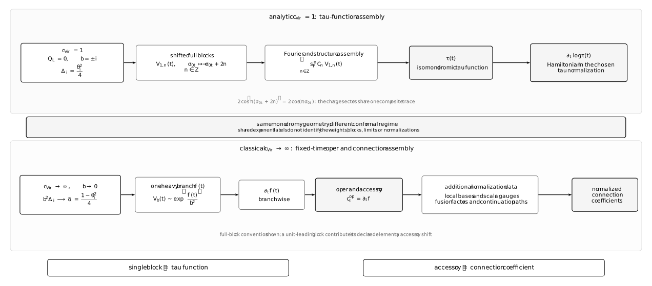
The two lanes share monodromy geometry but not a conformal regime. At $c_{\mathrm{Vir}}=1$, a shift family plus structure factors produces $\tau(t)$. At $c_{\mathrm{Vir}}\to\infty$, one classical branch produces an accessory coefficient; further normalization data are still needed for connection coefficients.

Shared monodromy geometry is not a block identity

Several objects legitimately carry across the two lanes:

• the modulus $t$ and the four-puncture character variety;
• local exponent differences and a lifted composite exponent;
• branch, channel, and scalar-versus-system conventions;
• Hamiltonian relations connecting tau derivatives to accessory coordinates in specified isomonodromic scalar reductions.

This common geometry explains why both block regimes appear in the same ODE problem. It does not identify their central charges, conformal weights, block normalizations, or limiting operations. In particular, one may relate an isomonodromic Hamiltonian to an oper accessory after a precise Lax reduction without equating the underlying $c=1$ and $c\to\infty$ blocks.

The scalar lift contributes a central sign

Chapter 5 uses a traceless-system lift with $\operatorname{tr}(M_0M_t)=2\cos(\pi\sigma_{0t})$. The natural normal-form scalar lift in Chapter 6 instead gives $-2\cos(\pi\theta_{0t})$. For the same ordered separating loop,

$$\sigma_{0t} \equiv 1\pm\theta_{0t} \pmod 2.$$

The minus sign records a central $-\mathbb I$ choice in the half-density scalar lift. The projective monodromy geometry agrees, but the two displayed matrix lifts must not be identified silently.

The remaining pages answer different questions

Use the rest of the chapter as a decision map:

Need	Continue to
Exact PVI $c=1$ Fourier expansion, structure factors, and charge lattice	Page 2
Classical block and accessory ledger at large central charge	Page 3
General-Heun connection matrices	Page 4
Irregular blocks and confluent-Heun connections	Page 5
All factors needed for normalized connection coefficients	Page 6
Frobenius resonance versus Zamolodchikov poles	Page 7
Recurrence comparison and numerical status checks	Page 8

The first three rows revisit earlier results only to standardize their normalizations for connection formulae. Pages 4–6 perform the actual assembly; pages 7–8 audit exceptional loci, independent recurrences, and the strength of each claim.

Common pitfalls

Setting $b=1$ to obtain $c=1$. In this convention $b=1$ gives $c_{\mathrm{Vir}}=25$. The analytic $c=1$ chart has $b=\pm\ii$.

Calling one c = 1 block the tau function. The tau function also requires the shift lattice, Fourier multiplier, structure factors, elementary prefactor, and branch data.

Treating a classical block as an ordinary finite-c block. It is the leading logarithmic action extracted from a scaled family of heavy blocks on a chosen branch.

Using one weight dictionary in both regimes. The monodromy label may be the same while $\Delta^{(1)}=\theta^2/4$ and $\delta=(1-\theta^2)/4$ play different roles.

Equating an accessory coefficient with a connection coefficient. The latter additionally needs local bases, scalar gauges, fusion factors, continuation paths, and normalization data.

Presenting the analytic c = 1 blocks as real-b unitary Liouville theory. This chapter uses analytically continued Virasoro blocks and does not make that physical identification.

Exercises

1. Locate the two central charges

Solve $Q_{\mathrm L}=0$ for $b$, and compare with the expansion of $c_{\mathrm{Vir}}$ as $b\to0$.

Solution

The equation

$$b+b^{-1}=0$$

gives $b^2=-1$, hence $b=\pm\ii$. By contrast,

$$c_{\mathrm{Vir}} = 6b^{-2}+13+6b^2,$$

which diverges as $b\to0$. The two regimes lie on different parts of the parameter chart.

2. Derive both weight dictionaries

Starting from $\Delta=Q_{\mathrm L}^2/4-a_{\mathrm L}^2$, derive the $c=1$ and classical formulas for an exponent difference $\theta$.

Solution

At $c=1$, choose $Q_{\mathrm L}=0$ and $a_{\mathrm L}=\ii\theta/2$. Then

$$\Delta^{(1)} = -\left( \frac{\ii\theta}{2} \right)^2 = \frac{\theta^2}{4}.$$

In the classical scaling, $bQ_{\mathrm L}\to1$ and $ba_{\mathrm L}\to\theta/2$, so

$$b^2\Delta \longrightarrow \frac14-\frac{\theta^2}{4} = \frac{1-\theta^2}{4}.$$

3. Check the composite shift lattice

Show that $\sigma_{0t}\mapsto\sigma_{0t}+2n$ preserves the composite trace but changes the lifted internal weight. Translate the result to the source variables $\rho=\sigma_{0t}/2$ and $\vartheta_i=\theta_i/2$.

Solution

Periodicity gives

$$\cos \left[ \pi \left( \sigma_{0t}+2n \right) \right] = \cos(\pi\sigma_{0t}).$$

Therefore $\operatorname{tr}(M_0M_t)=2\cos(\pi\sigma_{0t})$ is unchanged. However,

$$\Delta_{0t,n}^{(1)} = \frac{ \left( \sigma_{0t}+2n \right)^2 }{4}$$

depends on $n$. The Fourier sum runs over exponent lifts, not distinct unlifted trace values.

In source variables the same operation is $\rho\mapsto\rho+n$, and the channel exponent becomes

$$(\rho+n)^2 -\vartheta_0^2 -\vartheta_t^2.$$

Substituting the factor-of-two dictionary reproduces $\kappa_n$ on this page.

4. Route four common tasks

Which regime or later page should be used to compute a PVI tau function, an oper accessory, a normalized Heun connection matrix, and a resonant limit?

Solution

• Use the $c=1$ Fourier expansion on page 2 for the PVI tau function.
• Use the classical block and its derivative on page 3 for the oper accessory.
• Use the general-Heun matrix assembly on page 4 or the sectorial confluent-Heun analysis on page 5 together with the normalization assembly on page 6 for a normalized Heun connection matrix.
• Use page 7 for exceptional limits, where Frobenius logarithms and conformal-block poles are kept distinct.
• Use the recurrence tests and status ledger on page 8 to compare an assembled block coefficient with an independent ODE calculation and to classify the strength of a confluent claim.

5. Complete an accessory derivative

Starting from $c_t^{\mathrm{op}}=\partial_t f_{0t}$, list the additional data needed for a normalized zero-to-one connection coefficient.

Solution

One must also specify the two ordered local bases, their leading coefficients, scalar gauges, exponent lifts, branch cuts, continuation path, degenerate fusion or braiding factors, and any chiral-vertex or physical field normalization. The accessory determines the equation, not those normalized bases.

6. Classify the claims

Classify the following as exact, schematic, conditional, or not claimed: $b=\pm\ii$ at $c=1$; the displayed anatomy of the Fourier expansion; classical block exponentiation; and equality of the two block regimes.

Solution

The first statement is exact algebra. The displayed Fourier anatomy is schematic until page 2 fixes its elementary and structure factors. The classical exponentiation of a generic four-point block is established coefficientwise as a formal sewing-series statement. Continuing one branch and using it inside the derivative-compatible heavy–light factorization still requires the Chapter 6 regularity assumptions. Equality of the two regimes is not claimed.

References

• O. Gamayun, N. Iorgov, and O. Lisovyy, “Conformal Field Theory of Painlevé VI”, Journal of High Energy Physics 2012 (10), 038; see the erratum. Equations (1.8)–(1.12) state the originally conjectured $c=1$ Fourier-block expansion, structure factors, and second monodromy coordinate for PVI; the next two references give derivations and a proof in the generic setting.
• N. Iorgov, O. Lisovyy, and J. Teschner, “Isomonodromic Tau-Functions from Liouville Conformal Blocks”, Communications in Mathematical Physics 336 (2015), 671–694. Equations (4.43b)–(4.44) construct the PVI tau function from analytically continued Virasoro blocks; Section 7.2 explains the continuation to $c=1$ and why the Fourier transform is special there.
• P. Gavrylenko and O. Lisovyy, “Fredholm Determinant and Nekrasov Sum Representations of Isomonodromic Tau Functions”, Communications in Mathematical Physics 363 (2018), 1–58. Theorem B and equation (1.10) prove the generic charged partition series from a Fredholm determinant and identify its $c=1$ conformal-block form.
• A. Litvinov, S. Lukyanov, N. Nekrasov, and A. Zamolodchikov, “Classical Conformal Blocks and Painlevé VI”, Journal of High Energy Physics 2014 (7), 144. Equations (1.5)–(1.6) formulate the classical scaling and exponentiation ansatz; equations (2.6)–(2.14) derive the heavy–light BPZ reduction, accessory derivative, and monodromy consequences conditional on that asymptotic.
• M. Beşken, S. Datta, and P. Kraus, “Semi-Classical Virasoro Blocks: Proof of Exponentiation”, Journal of High Energy Physics 2020 (1), 109. Section 3 proves generic four-point exponentiation; page 3 separates this formal sewing-series result from the additional derivative and continuation assumptions.
• G. Bonelli, C. Iossa, D. Panea Lichtig, and A. Tanzini, “Irregular Liouville Correlators and Connection Formulae for Heun Functions”, Communications in Mathematical Physics 397 (2023), 635–727. Equations (3.1.22)–(3.1.28) provide the explicit normalized semiclassical heavy–light block-to-Heun reduction used in the second lane.