Recurrence Comparison, Numerical Tests, and Status Ledger

The safest comparison between a conformal block and an ODE recurrence does not identify their raw coefficients. A finite-$c$ Virasoro block coefficient aggregates descendants at level $N$; a classical logarithm is organized by coupling order $m$; and a Frobenius coefficient is indexed by a power $k$ of the independent variable. The objects become comparable only after each construction has produced the same normalized connection coefficient and both results have been expanded in the same weak-coupling parameter.

This page makes that principle executable for the general Heun equation. On the ODE side, the Schäfke–Schmidt theorem converts the large-order tail of one Frobenius series into an exact connection coefficient. A rescaling turns its recurrence into a stable three-term relation and a dual continued fraction. On the CFT side, a classical-block coefficient and accessory inversion predict the first weak-coupling coefficient. The two expressions agree; a reproducible high-precision test then checks the complete finite-$\lambda$ matrix, its determinant, its weak-coupling scaling, and forward–backward recurrence agreement.

What is actually compared

If

$$\log \frac{\mathsf C(\lambda)} {\mathsf C_{\mathrm{HG}}} = \sum_{m=1}^{\infty} f_m\lambda^m,$$

then the meaningful test is

$$f_m^{\mathrm{block}} = f_m^{\mathrm{ODE}}.$$

It is not an equality between a raw block or classical-log coefficient such as $\mathcal F_N$ or $\mathcal W_m$ and a Frobenius coefficient $u_k$. The three subscripts belong to different expansions.

Status of this page

Statement	Status
Schäfke–Schmidt extraction from large-order Frobenius coefficients	Theorem under the analytic and nonresonance hypotheses stated below
General-Heun three-term recurrence and continued fraction	Exact ODE-side result for the declared $\lvert t\rvert>1$ chart
Hypergeometric limit	Exact
First-order equality $f_1^{\mathrm{block}}=f_1^{\mathrm{ODE}}$	Exact meromorphic identity after the stated accessory inversion
General-Heun comparison at higher orders	Symbolically checked through $\lambda^3$ in Lisovyy–Naidiuk
All-orders equality with the classical-block formula	Formal or conjectural in the generality used here; not proved by the numerical test
Numerical matrix below	Reproducible observation with cutoff extrapolation and independent audits
Extension through resonance or a recurrence pole	Not supplied; use the limiting frames of page 7

Two recurrences use two different indices

Three integers appear in a practical comparison:

• $N$ is a Virasoro descendant level at finite central charge.
• $m$ is the order of the final weak-coupling series in $\lambda=t^{-1}$.
• $k$ is the Frobenius or Taylor order in the independent variable $z$.

The finite-$c$ block has the schematic expansion

$$\mathcal F(t) = \sum_{N=0}^{\infty} \mathcal F_N t^{-N}.$$

Its classical logarithm is reorganized as

$$\mathcal W(t) = \left( \delta_\infty-\delta_\sigma-\delta_t \right)\log t + \sum_{m=1}^{\infty} \mathcal W_m\lambda^m.$$

After the accessory relation has been inverted, the internal exponent $\sigma$ itself depends on $\lambda$. Fusion factors and endpoint derivatives must then be expanded as well. Only after this assembly does one obtain $f_m^{\mathrm{block}}$.

The ODE calculation begins instead with a normalized Taylor series

$$\widehat u(z) = \sum_{k=0}^{\infty}u_kz^k.$$

One solves a recurrence in $k$, takes a large-$k$ limit, and finally expands the resulting connection coefficient in $\lambda$. That last operation produces $f_m^{\mathrm{ODE}}$.

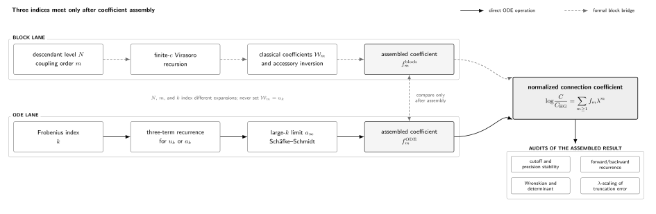
The Virasoro level $N$, coupling order $m$, and Frobenius order $k$ belong to different recurrences. The dashed comparison is made only between assembled coefficients of the same normalized connection coefficient; solid arrows denote exact ODE operations.

This separation is useful even when a computer algebra system hides the intermediate indices. It prevents an accidental “proof” obtained by matching two unrelated finite arrays.

Fix the Heun chart and every normalization

Use the normal form

$$\begin{aligned} 0={}& \psi''(z) + \Bigg[ \frac{\frac14-\theta_0^2}{z^2} + \frac{\frac14-\theta_1^2}{(z-1)^2} + \frac{\frac14-\theta_t^2}{(z-t)^2} \\ &+ \frac{ \theta_0^2+\theta_1^2+\theta_t^2 -\theta_\infty^2-\frac12 }{ z(z-1) } \\ &+ \frac{ (t-1) \left( \omega^2+\theta_t^2-\theta_\infty^2-\frac14 \right) }{ z(z-1)(z-t) } \Bigg]\psi(z), \end{aligned}$$

with

$$\lambda=\frac1t, \qquad |t|>1.$$

The parameter $\omega$ is the limiting composite exponent as $t\to\infty$; it is an accessory coordinate, not a fifth local exponent. At zero and one use the unit-leading normal-form germs

$$\begin{aligned} \psi_\pm^{[0]}(z) &= z^{\frac12\mp\theta_0} \left( 1+O(z) \right), \\ \psi_\pm^{[1]}(z) &= (1-z)^{\frac12\mp\theta_1} \left( 1+O(1-z) \right). \end{aligned}$$

For real $t>1$, take the powers real on $0<z<1$ and continue without winding around another puncture. The complex-$t$ formula is the analytic continuation of this branch inside the declared $|\lambda|<1$ chart. Assume

$$2\theta_0\notin\mathbb Z, \qquad 2\theta_1\notin\mathbb Z,$$

and avoid the gamma and recurrence poles displayed below. For the first-order block comparison, also assume

$$\omega\neq0, \qquad \omega^2\neq\frac14.$$

These are singular coordinates for the displayed accessory inversion; special limits require a different local parameter.

Write the source-first relation as

$$\psi_\epsilon^{[0]} = \sum_{\epsilon'=\pm} \mathsf C( \epsilon\theta_0, \epsilon'\theta_1 ) \psi_{\epsilon'}^{[1]}.$$

Thus the first sign labels a source row and the second a target column. In the book’s ordered row-frame convention $\boldsymbol H_0=\boldsymbol H_1C_{10}$,

$$C_{10} = \left( \mathsf C^{\mathrm{src}} \right)^{\mathsf T}.$$

The transpose does not change the determinant. Since

$$\begin{aligned} \operatorname{Wr} \left( \psi_+^{[0]},\psi_-^{[0]} \right) &= 2\theta_0, \\ \operatorname{Wr} \left( \psi_+^{[1]},\psi_-^{[1]} \right) &= -2\theta_1, \end{aligned}$$

the normalization audit is

$$\det\mathsf C^{\mathrm{src}} = \det C_{10} = -\frac{\theta_0}{\theta_1}.$$

Normalization ledger

Datum	Choice on this page
Equation	Displayed four-singularity normal form
Weak variable	$\lambda=t^{-1}$ with $\lvert\lambda\rvert<1$
Source and target	Unit-leading normal-form germs at $z=0$ and $z=1$
Ordering	Signs $(+,-)$ at both endpoints
Branch and path	Real powers on $0<z<1$ for $t>1$, then analytic continuation in the same chart
Matrix orientation	Literature array is source-first; the book’s target-row matrix is its transpose
Determinant	$-\theta_0/\theta_1$
Exclusions	$2\theta_0,2\theta_1\notin\mathbb Z$; no gamma pole; no static or dynamic recurrence denominator zero; for the block comparison, $\omega\neq0$ and $\omega^2\neq\frac14$
CFT dictionary	$\delta_\nu=\frac14-\nu^2$ and accessory inversion $\sigma(\lambda)\to\omega$
Mathematical status	Exact ODE theorem; finite-order classical-block comparison

Large Frobenius order isolates one connection coefficient

Gauge and normalize the $+$ source solution by

$$\begin{aligned} \widehat u(z) :={}& t^{\frac12-\theta_t} z^{-\frac12+\theta_0} (1-z)^{-\frac12-\theta_1} (t-z)^{-\frac12+\theta_t} \psi_+^{[0]}(z) \\ ={}& 1+\sum_{k=1}^{\infty}u_kz^k \end{aligned}$$

The only singularity of this Taylor series on the unit circle is the target point $z=1$. Darboux asymptotics therefore select the coefficient of the singular target branch. The modified Schäfke–Schmidt formula is

$$\mathsf C(\theta_0,\theta_1) = \Gamma(2\theta_1) (1-\lambda)^{\frac12-\theta_t} \lim_{k\to\infty} k^{1-2\theta_1}u_k.$$

This is the key ODE-side bridge. It turns a local series at zero into a global coefficient connecting zero to one. Its hypotheses matter: another singularity on or inside the unit circle, a resonant endpoint, or an undeclared branch can invalidate the simple limit.

At $\lambda=0$, the remaining equation is hypergeometric. Put

$$x = \frac12-\theta_0+\theta_1$$

and factor its coefficients from the finite-$\lambda$ coefficients:

$$\begin{aligned} h_k &= \frac{ (x+\omega)_k(x-\omega)_k }{ k!\,(1-2\theta_0)_k }, \\ u_k &= h_ka_k. \end{aligned}$$

The ratio $a_k$ satisfies

$$a_{k+1}-a_k = -\lambda \left( \alpha_ka_k+\beta_ka_{k-1} \right), \qquad a_{-1}=0, \quad a_0=1,$$

where

$$\alpha_k = - \frac{ \left( k+\frac12-\theta_0-\theta_t \right)^2 -\theta_0^2-\theta_\infty^2+\omega^2 }{ \left( k+\frac12-\theta_0+\theta_1 \right)^2-\omega^2 }, \qquad k\geq0,$$

and

$$\beta_k = \frac{ k(k-2\theta_0) \left[ \left( k-\theta_0+\theta_1-\theta_t \right)^2-\theta_\infty^2 \right] }{ D_kD_{k-1} }, \qquad k\geq1,$$

with

$$D_k = \left( k+\frac12-\theta_0+\theta_1 \right)^2-\omega^2.$$

Set $\beta_0:=0$ in the $k=0$ recurrence; its term multiplies $a_{-1}=0$ and the formula containing $D_{-1}$ is not used there. The recurrence chart excludes $D_k=0$ for $k\geq0$. The singularity can be removable in another parametrization, but direct substitution into this recurrence is not legitimate.

Stirling asymptotics of $h_k$ give

$$\mathsf C_{\mathrm{HG}} = \frac{ \Gamma(1-2\theta_0)\Gamma(2\theta_1) }{ \Gamma(x+\omega)\Gamma(x-\omega) }.$$

If $a_\infty=\lim_{k\to\infty}a_k$, then

$$\mathsf C(\theta_0,\theta_1) = \mathsf C_{\mathrm{HG}} (1-\lambda)^{\frac12-\theta_t} a_\infty.$$

Setting $\lambda=0$ makes $a_k=1$ for every $k$ and recovers the Gauss connection coefficient exactly.

The dual recurrence gives a stable continued fraction

A forward recurrence is conceptually direct, but extracting $a_\infty$ at high precision from an algebraic tail can be slow. The dual recurrence uses ratios $\eta_k$ satisfying

$$\eta_k = 1-\lambda\alpha_{k-1} -\frac{\lambda\beta_k}{\eta_{k+1}}, \qquad \eta_k\longrightarrow1 \quad(k\to\infty).$$

The exact limiting identity is

$$\log a_\infty = -\log(1-\lambda) + \sum_{k=1}^{\infty}\log\eta_k.$$

Combining the explicit power with $a_\infty$ gives the compact connection formula

$$\begin{aligned} \log \frac{ \mathsf C(\theta_0,\theta_1;\lambda) }{ \mathsf C_{\mathrm{HG}} } ={}& - \left( \frac12+\theta_t \right) \log(1-\lambda) \\ &+ \sum_{k=1}^{\infty} \log \left( 1-\lambda\alpha_{k-1} -\frac{\lambda\beta_k}{\eta_{k+1}} \right). \end{aligned}$$

Although $\alpha_k\to-1$ and $\beta_k\to1$, their first-order combination obeys

$$\alpha_{k-1}+\beta_k = O(k^{-2}).$$

That cancellation is why the coefficient sums converge. Summing $\alpha_k$ and $\beta_k$ separately is numerically and conceptually the wrong operation.

For complex $\lambda$, every logarithm in the truncated expression must be followed on one continuous branch. Exponentiating only at the end removes integer multiples of $2\pi\ii$ from the final coefficient, but it does not repair a continuation path that crosses a zero of some $\eta_k$.

The first assembled block coefficient matches the ODE sum

Define

$$\delta_\nu = \frac14-\nu^2.$$

The classical block in the $t\to\infty$ channel begins with

$$\mathcal W(t) = \left( \delta_\infty-\delta_\sigma-\delta_t \right)\log t + \mathcal W_1\lambda + O(\lambda^2),$$

where

$$\mathcal W_1 = \frac{ \left( \delta_\sigma-\delta_0+\delta_1 \right) \left( \delta_\sigma-\delta_\infty+\delta_t \right) }{ 2\delta_\sigma }.$$

The ODE is parametrized by $\omega$, whereas the block formula is parametrized by the composite monodromy exponent $\sigma$. Inverting the accessory relation gives

$$\sigma(\lambda) = \omega+\sigma_1\lambda+O(\lambda^2).$$

Introduce

$$\begin{aligned} A &= \frac14-\omega^2+\theta_0^2-\theta_1^2, \\ B &= \frac14-\omega^2+\theta_\infty^2-\theta_t^2. \end{aligned}$$

Then

$$\sigma_1 = \frac{ AB }{ 4\omega \left( \frac14-\omega^2 \right) }.$$

The fusion gamma factor must also be expanded at $\sigma(\lambda)$, and the classical endpoint derivatives contribute their own finite dressing. With $\psi_0$ denoting the digamma function, the assembled first coefficient is

$$\begin{aligned} f_1^{\mathrm{block}} ={}& - \frac{ AB }{ 4\omega \left( \frac14-\omega^2 \right) } \left[ \psi_0(x+\omega) -\psi_0(x-\omega) \right] \\ &- \frac{ (\theta_0+\theta_1)B }{ 2 \left( \frac14-\omega^2 \right) }. \end{aligned}$$

Expanding the exact continued fraction to first order instead gives

$$f_1^{\mathrm{ODE}} = \frac12+\theta_t - \sum_{k=1}^{\infty} \left( \alpha_{k-1}+\beta_k \right).$$

Partial fractions reduce the summand to rational tails and differences of simple poles. The latter use

$$\sum_{k=0}^{\infty} \left( \frac1{k+p}-\frac1{k+q} \right) = \psi_0(q)-\psi_0(p).$$

After simplification,

$$f_1^{\mathrm{ODE}} = f_1^{\mathrm{block}}.$$

Within the stated formal accessory inversion, this is an exact meromorphic coefficient identity, not merely a decimal match. It does not prove the accessory relation or the all-orders CFT-to-ODE correspondence. The ODE recurrence formula itself is exact at finite $\lambda$; the published ordinary-Heun comparison with the classical block was carried out symbolically through $\lambda^3$.

A rational slice exposes every audit

Choose

$$\begin{aligned} \theta_0&=\frac17, & \theta_1&=\frac29, & \theta_t&=\frac15, \\ \theta_\infty&=\frac3{11}, & \omega&=\frac25. \end{aligned}$$

No endpoint is resonant, the gamma factors are finite, and no $D_k$ vanishes. At 60 decimal digits the analytic quantities are

$$\begin{aligned} \mathsf C_{\mathrm{HG}} &= 0.4876551624635933898374010205783103148\ldots, \\ f_1 &= -0.5305332617596067437571423340270154671\ldots. \end{aligned}$$

For $\lambda=0.04$, the recurrence begins

$$\begin{aligned} a_0&=1, \\ a_1&= 1.02047217475176444105852\ldots, \\ a_2&= 0.996329805664173382742\ldots. \end{aligned}$$

These are ratios $a_k=u_k/h_k$, not block coefficients. The backward continued fraction gives

$$\mathsf C(\theta_0,\theta_1;0.04) = 0.4770670955559479494103401397381320146\ldots.$$

The first-order block approximation is

$$\mathsf C_{\mathrm{HG}} \exp(f_1\lambda) = 0.4774155049617878621\ldots.$$

The expected error is $O(\lambda^2)$. The scaling table makes that statement testable:

$\lambda$	Full recurrence	First-order block approximation	Relative error
$0.08$	$0.4659746313229458980$	$0.4673908571508970901$	$3.0393\times10^{-3}$
$0.04$	$0.4770670955559479494$	$0.4774155049617878621$	$7.3032\times10^{-4}$
$0.02$	$0.4824217403753359683$	$0.4825081715730616888$	$1.7916\times10^{-4}$
$0.01$	$0.4850533144443050368$	$0.4850748404096761558$	$4.4379\times10^{-5}$

Halving $\lambda$ reduces the relative error by approximately four, as an omitted quadratic term requires.

Flipping the two endpoint signs generates the complete source-first array:

$$\mathsf C^{\mathrm{src}} = \begin{pmatrix} 0.4770670955559479494 & 0.5961043904244732893 \\ 1.0355527564109983490 & -0.05357652724842792145 \end{pmatrix}.$$

Its determinant satisfies

$$\det\mathsf C^{\mathrm{src}} = -0.6428571428571428571429527\ldots,$$

whereas the Wronskian prediction is exactly

$$-\frac{\theta_0}{\theta_1} = -\frac9{14}.$$

The raw determinant residual in the default extrapolation is $9.55\times10^{-23}$. Raw forward–backward differences for all four entries are at most $2\times10^{-22}$. These small consistency residuals are not certified error bounds: correlated cutoff errors can cancel. The printed last-diagonal changes and reruns at larger cutoffs remain the convergence diagnostics.

Reproduce the calculation

The audit script uses Python 3.10.16 and mpmath 1.3.0. Run

python3 public/code/advanced-ode/heun-recurrence-block-check.py \
  --show-matrix --show-scaling --check-forward

The default maximum Frobenius orders are $K_{\max}=128,256,\ldots,8192$. The program prints the raw cutoff values, ordinary Richardson diagonals for the expected inverse-$K_{\max}$ tail, and the last diagonal change. It also validates $|\lambda|<1$, endpoint resonance, gamma poles, recurrence poles, and dynamic continued-fraction denominators.

The last printed digits should not be interpreted independently of the cutoff table. Increasing --dps without increasing --base-cutoff or --levels improves arithmetic but does not remove a truncation tail.

What survives at each confluent level

The phrase “the conformal-block connection formula” hides several different mathematical statements. A regular-to-regular coefficient can sometimes be reached by a large-order Taylor theorem. A regular-to-irregular coefficient additionally requires a sectorial normalization. An irregular-to-irregular matrix requires both endpoint sectors and Stokes data. Accessory expansions alone do not supply any of those missing frames.

Equation and endpoints	Direct ODE control used in this chapter	Block-side evidence	Current claim
Hypergeometric, regular–regular	Classical gamma connection theorem	Degenerate rigid fusion kernel	Exact normalized coefficient
General Heun, regular–regular, $\lvert t\rvert>1$	Schäfke–Schmidt theorem and exact continued fraction	Classical-block comparison through $\lambda^3$	ODE formula exact; CFT equality formal beyond checked orders
Confluent Heun, regular–regular, weak coupling	Direct recurrence/continued-fraction theorem	Irregular-block construction and perturbative agreement	Established ODE chart; block interpretation carries its semiclassical assumptions
Reduced confluent Heun, regular–regular	Direct recurrence/continued-fraction theorem	Comparison through $\lambda^5$	ODE formula exact; strongest finite-order block check in the 2022 analysis
Confluent Heun, regular–rank-one irregular	Exact endpoint kernels plus sector data	First- and second-kind irregular blocks	Sector-dependent, conditional classical assembly; no comparably general ODE-side theorem is used here
Doubly confluent Heun, rank-one irregular–rank-one irregular	Local formal recurrences and Stokes constraints	Irregular-block and collision constructions	Formal or conditional; a full normalized recurrence audit remains to be supplied
Reduced and doubly reduced DCHE variants	Parameter reductions and formal recurrences	Corresponding irregular limits	Same limitation; these reductions are not the biconfluent or triconfluent classes
Biconfluent Heun, regular–rank-two irregular	Accessory and sectorial asymptotics	Higher-rank irregular block proposals	Accessory-level evidence; no full normalized matrix audited here
Triconfluent Heun, one rank-three irregular point	Formal WKB and Stokes geometry	Higher-rank irregular or quantum-period proposals	Accessory or intersectorial Voros-level evidence; full Stokes matrix open here
Reduced biconfluent and reduced triconfluent variants	Formal normal forms and accessory recurrences	Candidate classical irregular blocks	Conjectural accessory/Voros correspondence checked at low orders; no normalized matrix audited here
$c=1$ PVI tau-function Fourier family	Isomonodromic theorem on its generic chart	Complete analytic $c=1$ blocks	Exact tau-function representation, but a different regime and output

Two cautions govern the table.

First, a confluence can preserve a theorem only after all gauges, branches, parameter scalings, and endpoint normalizations have controlled limits. A formal limit of the differential operator alone does not prove convergence of its connection matrix.

Second, the May 2026 preprint by Iwaki, Nagoya, and Shukuta derives formal accessory-parameter expansions across Heun confluences and formulates a candidate classical-irregular-block correspondence, tested at low orders. That broadens the evidence for the accessory-level dictionary; it does not by itself turn every regular-to-irregular or irregular-to-irregular normalized connection matrix into a proved analytic theorem.

A reusable comparison workflow

1. Declare the output. Decide whether the target is an accessory, one connection entry, a complete matrix, a Stokes multiplier, or a tau function.
2. Freeze the ODE frame. State the normal form, unit-leading local powers, branches, source–target direction, path, and sector.
3. Separate the indices. Name the descendant level, coupling order, and Frobenius order differently.
4. Invert the accessory relation. Express the block’s internal monodromy coordinate in the ODE’s fixed accessory coordinate before comparing coefficients.
5. Assemble before comparing. Include fusion gamma factors, classical derivative dressings, explicit powers, and frame conversions.
6. Compute the ODE coefficient independently. Use a Frobenius recurrence, continued fraction, Wronskian match, or direct integration.
7. Audit more than one scalar. Check a determinant, a limiting equation, convergence with cutoff, and—when possible—both recurrence directions.
8. Label the strongest justified status. Distinguish a theorem, finite-order formal equality, numerical observation, conditional sectorial statement, and conjecture.

This workflow is deliberately stricter than matching a few decimal coefficients. A normalization error can preserve the differential equation and even one matrix entry while violating the Wronskian law.

Common pitfalls

Comparing $u_k$ with $\mathcal W_k$. The former is a Taylor coefficient in $z$; the latter is a coupling coefficient after a classical limit. Compare the assembled $f_m$ instead.

Holding $\sigma$ fixed when the ODE holds $\omega$ fixed. The accessory relation makes $\sigma=\omega+\sigma_1\lambda+\cdots$. Omitting this inversion loses the digamma contribution to $f_1$.

Summing two divergent-looking pieces separately. The convergent tail is $\alpha_{k-1}+\beta_k=O(k^{-2})$, although $\alpha_k\to-1$ and $\beta_k\to1$. Preserve the cancellation before numerical summation.

Calling a finite-order check an all-orders proof. Agreement through $\lambda^3$ or $\lambda^5$ is strong evidence and a valuable error detector. It does not establish convergence, analytic continuation, or equality outside the common formal chart.

Using the source-first array as the book’s row-frame matrix. The literature relation lists source solutions by rows. The matrix in $\boldsymbol H_0=\boldsymbol H_1C_{10}$ is its transpose.

Trusting precision without cutoff control. More working digits do not cure an algebraic recurrence tail. Print a cutoff ladder and compare independent algorithms.

Exercises

1. Recover the hypergeometric limit

Set $\lambda=0$ in the recurrence for $a_k$. Show that $a_k=1$ and recover $\mathsf C_{\mathrm{HG}}$ from the Schäfke–Schmidt limit.

Solution

At $\lambda=0$,

$$a_{k+1}-a_k=0.$$

Since $a_0=1$, induction gives $a_k=1$. Therefore $u_k=h_k$. The gamma-ratio asymptotic

$$\frac{ \Gamma(k+x+\omega)\Gamma(k+x-\omega) }{ \Gamma(k+1)\Gamma(k+1-2\theta_0) } \sim k^{2\theta_1-1}$$

together with the fixed Pochhammer prefactors gives

$$\Gamma(2\theta_1) \lim_{k\to\infty} k^{1-2\theta_1}h_k = \mathsf C_{\mathrm{HG}}.$$

The factor $(1-\lambda)^{1/2-\theta_t}$ is one at $\lambda=0$.

2. Expand the continued fraction once

Use $\eta_k=1+O(\lambda)$ to derive $f_1^{\mathrm{ODE}}$ from the exact logarithmic formula.

Solution

To first order,

$$\eta_k = 1-\lambda \left( \alpha_{k-1}+\beta_k \right) +O(\lambda^2).$$

Hence

$$\log\eta_k = -\lambda \left( \alpha_{k-1}+\beta_k \right) +O(\lambda^2).$$

Also,

$$- \left( \frac12+\theta_t \right) \log(1-\lambda) = \left( \frac12+\theta_t \right)\lambda +O(\lambda^2).$$

Adding the terms gives

$$f_1^{\mathrm{ODE}} = \frac12+\theta_t - \sum_{k=1}^{\infty} \left( \alpha_{k-1}+\beta_k \right).$$

3. Convert matrix orientations

Starting from the source-first equations

$$\psi_i^{[0]} = \sum_j \mathsf C_{ij}^{\mathrm{src}} \psi_j^{[1]},$$

derive the matrix used in $\boldsymbol H_0=\boldsymbol H_1C_{10}$.

Solution

The $i$th component of the row vector $\boldsymbol H_1C_{10}$ is

$$\sum_j \psi_j^{[1]} (C_{10})_{ji}.$$

Comparison with the source-first equation requires

$$(C_{10})_{ji} = \mathsf C_{ij}^{\mathrm{src}}.$$

Therefore

$$C_{10} = \left( \mathsf C^{\mathrm{src}} \right)^{\mathsf T}.$$

4. Diagnose the scaling table

Let

$$\mathsf C(\lambda) = \mathsf C_{\mathrm{HG}} \exp \left( f_1\lambda+f_2\lambda^2+O(\lambda^3) \right).$$

Explain why the relative error of the first-order approximation falls by a factor approaching four when $\lambda$ is halved.

Solution

The approximation keeps $\mathsf C_{\mathrm{HG}}\exp(f_1\lambda)$, so the ratio of the exact answer to the approximation is

$$\exp \left( f_2\lambda^2+O(\lambda^3) \right) = 1+f_2\lambda^2+O(\lambda^3).$$

Thus the relative error is quadratic to leading order. Replacing $\lambda$ by $\lambda/2$ multiplies that leading term by $1/4$.

5. Find the static recurrence poles

Show that $D_k=0$ for a nonnegative integer $k$ exactly when one of $-x+\omega$ or $-x-\omega$ is a nonnegative integer.

Solution

Factor

$$D_k = (k+x-\omega)(k+x+\omega).$$

It vanishes when

$$k=-x+\omega \qquad\text{or}\qquad k=-x-\omega.$$

Requiring $k\in\mathbb Z_{\geq0}$ gives the stated criterion. This is a pole of the chosen rescaled recurrence chart, not automatically a Frobenius resonance at zero or one.

References

• R. Schäfke and D. Schmidt, “The Connection Problem for General Linear Ordinary Differential Equations at Two Regular Singular Points with Applications in the Theory of Special Functions”, SIAM Journal on Mathematical Analysis 11 (1980), 848–862. Proves the large-order connection principle used here.
• O. Lisovyy and A. Naidiuk, “Perturbative Connection Formulas for Heun Equations”, Journal of Physics A: Mathematical and Theoretical 55 (2022), 434005; arXiv:2208.01604. Theorem B gives the general-Heun recurrence and continued fraction; the paper compares ordinary-Heun block coefficients through $\lambda^3$ and reduced-confluent coefficients through $\lambda^5$.
• G. Bonelli, C. Iossa, D. Panea Lichtig, and A. Tanzini, “Irregular Liouville Correlators and Connection Formulae for Heun Functions”, Communications in Mathematical Physics 397 (2023), 635–727; arXiv:2201.04491. Develops the regular and irregular block connection constructions whose normalization data were assembled on pages 4–6.
• O. Lisovyy and A. Naidiuk, “Accessory Parameters in Confluent Heun Equations and Classical Irregular Conformal Blocks”, Letters in Mathematical Physics 111 (2021), 137. Gives perturbative accessory expansions and their irregular-block interpretation for confluent equations.
• K. Iwaki, H. Nagoya, and H. Shukuta, “Accessory Parameter of Confluent Heun Equations, Voros Periods and Classical Irregular Conformal Blocks”, preprint, May 2026. Derives formal accessory series and formulates a candidate block correspondence tested at low orders; it is cited here with the narrower status stated in the ledger.
• NIST Digital Library of Mathematical Functions, §31.12, “Confluent Forms of Heun’s Equation”. Fixes the confluence taxonomy and prevents reduced DCHE variants from being confused with the biconfluent and triconfluent equations.

Chapter 8 now replaces large Frobenius order by an $\hbar$-asymptotic recursion in formal WKB geometry. Return to the Chapter 7 map when the problem instead calls for the $c=1$ tau-function or classical-block route.