Stage B: Voros Symbols, Stokes Automorphisms, and Wall Crossing

Page 4 supplied the universal local shear across one Stokes edge. A route through several regions also changes normalization endpoints, and those changes contribute exponentials of regularized WKB periods. The formal exponentials are Voros symbols. Their directional Borel sums are analytic multiplicative coordinates attached to a summation chamber.

At a graph wall, one of the actions becomes a singular Borel direction. If the central graph actually contains the corresponding saddle trajectory, the two lateral coordinates differ by a birational automorphism. For one ordinary zero-to-zero saddle, that automorphism is the Delabaere–Dillinger–Pham, or DDP, transformation

$$\begin{aligned} \widehat{\mathcal X}_\beta &\longmapsto \widehat{\mathcal X}_\beta \left( 1+\widehat{\mathcal V}_\delta \right)^{-\langle\delta,\beta\rangle}, \\ \widehat{\mathcal V}_\gamma &\longmapsto \widehat{\mathcal V}_\gamma \left( 1+\widehat{\mathcal V}_\delta \right)^{-\delta\mathbin{\cdot}\gamma}. \end{aligned}$$

The active class $\delta$ must be oriented, the two intersection pairings must be ordered, and the lateral signs must be translated before this formula is used. The transformation is not a local Airy matrix, not the geometric flip of a preferred graph basis, and not a boundary condition.

Page question

How do regularized WKB periods become analytic multiplicative coordinates, and how does a realized saddle wall transform those coordinates while the underlying differential equation and its monodromy remain fixed?

Status ledger

Statement used on this page	Status
Additivity of regularized exponents and multiplicativity of their exponentials	Exact formal identities for compatible representatives and endpoint data
Factoring the classical exponential before ordinary Borel transformation	Required by the power-series Borel convention of Page 1
Existence of directional or lateral Voros symbols	Theorem only under the stated continuation, growth, path, endpoint, and uniformity hypotheses
Page 4’s diagonal transport after Borel summation	Exact once a continuous half-exponent is fixed
Phase alignment of an action implies a graph wall	False; the saddle trajectory must be geometrically realized
Ordinary DDP formula	Published theorem in its polynomial scope and in stated meromorphic extensions with their analytic input
The active saddle symbol does not jump	Exact consequence of $\delta\mathbin{\cdot}\delta=0$
Graph flip equals Stokes automorphism	False; a cluster-coordinate mutation combines a geometric basis change with an analytic jump
Simple-pole wall factor	Exact in the restricted meromorphic $R_0+\hbar^2R_2$ framework stated below
Double-pole loop formula	Exact in the standard pop framework with its projective pole and summability assumptions
Weber Borel-pole lattice and gamma calibration	Exact for the stated regularized path and compatible branches; summing the full lateral residue tower also requires the stated convergence control
Arbitrarily ordered products for several coupled saddles	False
A factor $1+\mathcal V_\delta$ supplies a spectrum by itself	False; boundary subspaces enter on Page 6

Four layers sit between a period and an analytic coordinate

Retain Chapter 8’s branch-difference form

$$\Omega(\hbar) = P_{\mathrm{even}}(z,\hbar)\,\dd z$$

and let $\gamma$ be an oriented closed cycle on the normalized WKB cover. Its formal quantum period, total Voros exponent, and classical-subtracted exponent are

$$\begin{aligned} \widehat\Pi_\gamma &:= \oint_\gamma\Omega(\hbar), \\ \widehat V_\gamma^{\mathrm{tot}} &:= \frac{\widehat\Pi_\gamma}{\hbar}, \\ Z_\gamma &:= \oint_\gamma\lambda_0, \\ \widehat V_\gamma^{\mathrm q} &:= \frac1\hbar \oint_\gamma \left( \Omega-\lambda_0 \right). \end{aligned}$$

Thus

$$\widehat V_\gamma^{\mathrm{tot}} = \frac{Z_\gamma}{\hbar} + \widehat V_\gamma^{\mathrm q}.$$

In the standard even-$\hbar$ setting,

$$\begin{aligned} \widehat\Pi_\gamma &= \sum_{k\geq0} \Pi_{\gamma,2k}\hbar^{2k}, \\ \widehat V_\gamma^{\mathrm q} &= \sum_{k\geq1} \Pi_{\gamma,2k}\hbar^{2k-1}. \end{aligned}$$

The formal cycle Voros symbol is

$$\widehat{\mathcal V}_\gamma := \exp\!\left( \widehat V_\gamma^{\mathrm{tot}} \right).$$

This notation lives in a completed transseries algebra. The factor $\exp(Z_\gamma/\hbar)$ is declared as a classical transmonomial; it is not passed through the ordinary power-series Borel transform. Only $\widehat V_\gamma^{\mathrm q}$ is treated by the shifted Borel transform of Page 1.

When the quantum correction is laterally summable and exponentiation is valid in the chosen summability algebra, define

$$\begin{aligned} \mathcal V_{\gamma,\theta\pm} :={}& \exp\!\left( \frac{Z_\gamma}{\hbar} \right) \\ &\times \exp\!\left( \mathcal S_{\theta\pm} \widehat V_\gamma^{\mathrm q} \right). \end{aligned}$$

This is an analytic function on the common $\hbar$-sector of the lateral sums. It is not the formal object $\widehat{\mathcal V}_\gamma$, even though the analytic function has that symbol as its asymptotic expansion.

The four layers are therefore

Layer	Object	Category
Period	$\widehat\Pi_\gamma$	Formal additive series
Exponent	$\widehat V_\gamma^{\mathrm{tot}}$	Formal Laurent/transseries exponent
Symbol	$\widehat{\mathcal V}_\gamma$	Formal multiplicative object
Sectorial symbol	$\mathcal V_{\gamma,\theta\pm}$	Analytic lateral Borel sum

Calling all four objects a “Voros coefficient” hides exactly the distinction needed at a wall.

Relative-path symbols use a different regularization

Let $\widehat P_0$ be the lifts of the zeros and let $\widehat P_\infty$ be the lifts of poles of order at least two. Set

$$\widehat P := \widehat P_0\cup\widehat P_\infty.$$

In the ordinary Iwaki–Nakanishi framework, the cycle and path groups are

$$\begin{aligned} \Gamma &= H_1 \left( \widehat\Sigma\setminus\widehat P; \mathbb Z \right), \\ \Gamma^\vee &= H_1 \left( \widehat\Sigma\setminus\widehat P_0, \widehat P_\infty; \mathbb Z \right). \end{aligned}$$

For a relative class $\beta\in\Gamma^\vee$, with all endpoint coordinates, subtraction scales, logarithm branches, and tangential directions fixed, put

$$\begin{aligned} \widehat W_\beta^{\mathrm q} &:= \frac1\hbar \int_\beta^{\mathrm{reg}} \left( \Omega-\lambda_0 \right), \\ \widehat{\mathcal X}_\beta &:= \exp\!\left( \widehat W_\beta^{\mathrm q} \right). \end{aligned}$$

The corresponding lateral analytic symbol is

$$\mathcal X_{\beta,\theta\pm} := \exp\!\left( \mathcal S_{\theta\pm} \widehat W_\beta^{\mathrm q} \right).$$

This path symbol is quantum-only. It is not the turning-point-to- turning-point action of Chapter 8. The latter closes to an anti-invariant cycle and naturally contributes a half-power of a total cycle symbol.

If a total open transport is needed and its classical endpoint normalization has been declared, keep it visibly separate:

$$\widehat{\mathcal T}_\beta := \exp\!\left( \frac{\mathcal A_\beta^{(0)}}{\hbar} \right) \widehat{\mathcal X}_\beta.$$

For compatible representatives and endpoint data,

$$\widehat{\mathcal T}_{\beta+\gamma} = \widehat{\mathcal T}_\beta \widehat{\mathcal V}_\gamma.$$

By contrast, adding $\gamma$ to the quantum-only path exponent adds only $\widehat V_\gamma^{\mathrm q}$, not the classical factor $\exp(Z_\gamma/\hbar)$.

When simple poles are admitted, write $\widehat P_s$ for their lifts and set

$$\widehat P^{(s)} := \widehat P_0 \cup \widehat P_s \cup \widehat P_\infty.$$

Both groups must then be updated:

$$\begin{aligned} \Gamma_s &:= H_1 \left( \widehat\Sigma\setminus\widehat P^{(s)}; \mathbb Z \right), \\ \Gamma_s^\vee &:= H_1 \left( \widehat\Sigma \setminus \left( \widehat P_0\cup\widehat P_s \right), \widehat P_\infty; \mathbb Z \right). \end{aligned}$$

The odd WKB form vanishes on deck-invariant classes, so many sources quotient by the invariant subgroup. Chapter 8 instead retained an explicit integral lattice. These descriptions agree only after the factor-of-two convention has been translated.

Multiplicative algebra remembers orientation

For compatible cycles,

$$\begin{aligned} \widehat{\mathcal V}_{\gamma+\rho} &= \widehat{\mathcal V}_\gamma \widehat{\mathcal V}_\rho, \\ \widehat{\mathcal V}_{-\gamma} &= \widehat{\mathcal V}_\gamma^{-1}, \\ \widehat{\mathcal V}_0 &= 1. \end{aligned}$$

The same laws hold for sectorial sums in a common chamber. Relative path composition is multiplicative only when the intermediate endpoint data match. A formal exponential does not erase a mismatch of local coordinates or subtraction constants.

Put oriented representatives in transverse position. This page uses

$$\langle\,\cdot,\cdot\,\rangle: \Gamma\times\Gamma^\vee \longrightarrow \mathbb Z$$

for cycle–path intersection and

$$\gamma\mathbin{\cdot}\rho$$

for cycle–cycle intersection. A crossing contributes $+1$ when the ordered tangent of the first curve followed by that of the second curve agrees with the complex orientation of the cover. Hence

$$\gamma\mathbin{\cdot}\rho = -\rho\mathbin{\cdot}\gamma.$$

The active saddle cycle will always be the first argument in a jump exponent. Reversing the two entries changes the sign.

Away from a singular Borel direction, there is one ordinary directional sum. In that case this page suppresses the lateral sign and writes $\mathcal V_{\gamma,\theta}$ rather than $\mathcal V_{\gamma,\theta\pm}$.

Page 4’s diagonal transport becomes analytic

Suppose the lifted path between two ramified normalization endpoints closes to the anti-invariant cycle $\gamma$. Page 4 obtained the formal frame relation

$$\widehat F_a = \widehat F_b \begin{pmatrix} \exp(\widehat V_\gamma^{\mathrm{tot}}/2)&0 \\ 0&\exp(-\widehat V_\gamma^{\mathrm{tot}}/2) \end{pmatrix}.$$

After summation in one chamber,

$$\begin{aligned} F_a^\theta &= F_b^\theta D_{\gamma,\theta}, \\ D_{\gamma,\theta} &= \begin{pmatrix} \mathcal V_{\gamma,\theta}^{1/2}&0 \\ 0&\mathcal V_{\gamma,\theta}^{-1/2} \end{pmatrix}. \end{aligned}$$

The half-power means the exponential of half the continuously summed exponent. It is not an unrelated numerical square root chosen after the fact.

With Page 4’s matrices

$$L(\kappa) = \begin{pmatrix} 1&0\\ \kappa&1 \end{pmatrix}, \qquad U(\kappa) = \begin{pmatrix} 1&\kappa\\ 0&1 \end{pmatrix},$$

diagonal transport gives

$$\begin{aligned} D_{\gamma,\theta}^{-1} L(\ii) D_{\gamma,\theta} &= L\!\left( \ii\mathcal V_{\gamma,\theta} \right), \\ D_{\gamma,\theta}^{-1} U(\ii) D_{\gamma,\theta} &= U\!\left( \ii\mathcal V_{\gamma,\theta}^{-1} \right). \end{aligned}$$

The local multiplier $\ii$ and the nonlocal Voros factor therefore have different origins. This matrix calculation motivates the form of global connection products, but it is not a proof of the DDP theorem.

A wall requires a realized saddle trajectory

Fix a central Borel direction $\theta_0$. Assume that the phased graph $G_{\theta_0}$ contains a regular saddle trajectory $\ell_0$ joining two distinct simple zeros. Let $\delta$ be its lifted saddle class, oriented by

$$\ee^{-\ii\theta_0}Z_\delta \in \mathbb R_{<0}.$$

Equivalently, define the positive Borel action

$$\omega_\delta := -Z_\delta \in L_{\theta_0}.$$

For $\hbar$ in the compatible decay sector,

$$\widehat{\mathcal V}_\delta \sim \exp\!\left( -\frac{\omega_\delta}{\hbar} \right)$$

is exponentially small. This orientation is part of the theorem. A cycle orientation inherited from a previously drawn branch cut need not be the active orientation.

The phase test

$$\operatorname{Im} \left( \ee^{-\ii\theta_0}Z_\delta \right) = 0$$

is necessary for a saddle trajectory of class $\delta$, but Page 3 showed that it is not sufficient. The horizontal representative $\ell_0$ must actually exist.

For the ordinary theorem used below, assume more precisely:

• the equation is in Schrödinger normal form on a compact connected Riemann surface, with meromorphic coefficients satisfying the stated exact-WKB pole-growth and projective double-pole conditions;
• the leading quadratic differential has simple zeros, poles of order at least two, and no recurrent trajectories;
• the central graph has exactly one regular saddle trajectory and no coalescing critical points;
• sufficiently small rotations on both sides are saddle-free;
• cycles and paths are identified by Gauss–Manin transport;
• the required cycle and path symbols admit the two uniform lateral sums.

The original DDP proof treats an $\hbar$-independent polynomial potential. Iwaki–Nakanishi’s Theorem 3.4 gives the meromorphic formulation above, with its cited summability input. The formula is not being asserted here for a higher-order turning point, a multiple simultaneous saddle, or an arbitrary formal potential without a summability theorem.

The DDP theorem turns intersection into a jump

The regular zero-to-zero wall is conventionally called a type-I wall. Define its fixed-lattice formal automorphism $\mathfrak S_\delta^{\mathrm I}$ by

$$\begin{aligned} \mathfrak S_\delta^{\mathrm I} \left( \widehat{\mathcal X}_\beta \right) &= \widehat{\mathcal X}_\beta \left( 1+\widehat{\mathcal V}_\delta \right)^{-\langle\delta,\beta\rangle}, \\ \mathfrak S_\delta^{\mathrm I} \left( \widehat{\mathcal V}_\gamma \right) &= \widehat{\mathcal V}_\gamma \left( 1+\widehat{\mathcal V}_\delta \right)^{-\delta\mathbin{\cdot}\gamma}. \end{aligned}$$

Page 2 fixed the operational Stokes convention

$$\mathcal S_{\theta_0+} = \mathcal S_{\theta_0-} \circ \mathfrak S_\delta^{\mathrm I}.$$

Therefore the analytic DDP formula in this book is

$$\begin{aligned} \mathcal X_{\beta,\theta_0+} ={}& \mathcal X_{\beta,\theta_0-} \\ &\times \left( 1+\mathcal V_{\delta,\theta_0-} \right)^{-\langle\delta,\beta\rangle}, \\ \mathcal V_{\gamma,\theta_0+} ={}& \mathcal V_{\gamma,\theta_0-} \\ &\times \left( 1+\mathcal V_{\delta,\theta_0-} \right)^{-\delta\mathbin{\cdot}\gamma}. \end{aligned}$$

The lower lateral value appears on the right. Iwaki–Nakanishi use a large parameter $\eta=1/\hbar$ and phase $\alpha=-\theta$. Their printed lateral labels translate as

$$\begin{aligned} \mathcal S_{\theta+}^{\mathrm{book}} &= \mathcal S_-^{\mathrm{IN}}, \\ \mathcal S_{\theta-}^{\mathrm{book}} &= \mathcal S_+^{\mathrm{IN}}. \end{aligned}$$

Thus their relation

$$\mathcal S_-^{\mathrm{IN}} = \mathcal S_+^{\mathrm{IN}} \circ \mathfrak S_\delta$$

becomes exactly the book’s operational equation above. Copying the subscripts without translating $\eta=1/\hbar$ reverses the jump.

Several checks are immediate.

• The active symbol is unchanged because $\delta\mathbin{\cdot}\delta=0$.
• A path or cycle disjoint from $\delta$ does not jump.
• If $\langle\delta,\beta\rangle=1$, the path symbol is divided by $1+\mathcal V_\delta$.
• If $\delta\mathbin{\cdot}\gamma=-1$, the cycle symbol is multiplied by $1+\mathcal V_\delta$.
• Crossing the same wall in the reverse direction uses $(\mathfrak S_\delta^{\mathrm I})^{-1}$.

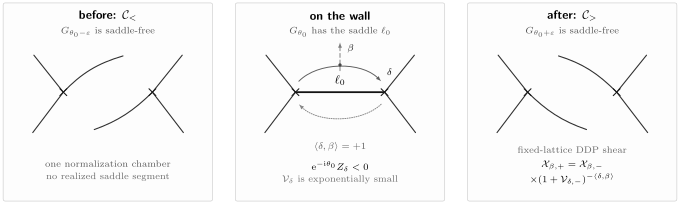
A realized saddle wall has two distinct effects. The spatial Stokes graph changes its resolution, while fixed-lattice Voros coordinates undergo the DDP intersection shear. A graph-adapted coordinate mutation combines this analytic automorphism with the separate change of preferred cycle and path basis.

Weber calibrates one active wall exactly

For the Weber curve of Pages 3 and 8,

$$R_0(z) = z^2-a^2, \qquad a>0,$$

the displayed cut cycle $\delta_{\mathrm{cut}}$ has

$$Z_{\delta_{\mathrm{cut}}} = \ii\pi a^2.$$

At the wall angle $\theta_0=\pi/2$, the DDP orientation is the opposite one:

$$\begin{aligned} \delta &= -\delta_{\mathrm{cut}}, \\ Z_\delta &= -\ii\pi a^2. \end{aligned}$$

Every higher closed Weber period vanishes. On the central ray $\hbar=\ii|\hbar|$, the active symbol is therefore exactly

$$q := \mathcal V_\delta = \exp\!\left( -\frac{\pi a^2}{|\hbar|} \right).$$

For a relative path with $\langle\delta,\beta\rangle=1$,

$$\mathcal X_{\beta,+} = \frac{ \mathcal X_{\beta,-} }{ 1+q }.$$

After a continuous logarithm branch is fixed, put

$$\Delta_\beta := \Log\mathcal X_{\beta,+} - \Log\mathcal X_{\beta,-}.$$

Then

$$\begin{aligned} \Delta_\beta &= -\Log(1+q) \\ &= -q +\frac{q^2}{2} -\frac{q^3}{3} +\cdots. \end{aligned}$$

One primitive saddle action thus generates a complete tower of exponentially small action grades. The terms $q^n$ are composites in the automorphism; the expansion does not declare every $n\delta$ to be a new primitive saddle trajectory.

The relative Weber coefficient sees the Borel-pole lattice

The closed Weber period is classical, but Page 8’s regularized path $\beta_{\mathrm W}:\infty_-\to\infty_+$ has a nonzero quantum exponent. Put

$$\mu := \frac{a^2}{2}.$$

With the path orientation for which $\langle\delta,\beta_{\mathrm W}\rangle=-1$, its formal exponent is

$$\widehat W_{\mathrm W}(\hbar) = \sum_{k\geq1} \frac{ \left(2^{1-2k}-1\right)B_{2k} }{ 2k(2k-1)\mu^{2k-1} } \hbar^{2k-1}.$$

Its shifted Borel transform can be summed at the level of germs:

$$\begin{aligned} \mathcal B\widehat W_{\mathrm W}(\xi) ={}& \frac{1}{2\xi} \left[ \frac{1}{\ee^{\xi/(2\mu)}-1} \right. \\ &\left. + \frac{1}{\ee^{\xi/(2\mu)}+1} - \frac{2\mu}{\xi} \right]. \end{aligned}$$

The apparent singularity at $\xi=0$ is removable. The nonzero poles on the imaginary lattice are

$$\xi_k = 2\pi\ii\mu k = \pi\ii a^2k, \qquad k\in\mathbb Z\setminus\{0\},$$

with residues

$$\operatorname*{Res}_{\xi=\xi_k} \mathcal B\widehat W_{\mathrm W} = \frac{(-1)^k}{2\pi\ii k}.$$

At $\theta_0=\pi/2$, the positive poles contribute Laplace weights $q^k$. Page 2’s upper-minus-lower indentation convention supplies $-2\pi\ii$ times each residue. Hence

$$\begin{aligned} \mathcal S_{\theta_0+}\widehat W_{\mathrm W} - \mathcal S_{\theta_0-}\widehat W_{\mathrm W} &= \sum_{k\geq1} \frac{(-1)^{k+1}}{k}q^k \\ &= \Log(1+q). \end{aligned}$$

Exponentiating yields

$$\mathcal X_{\beta_{\mathrm W},+} = \mathcal X_{\beta_{\mathrm W},-} (1+q),$$

exactly as DDP predicts from $-\langle\delta,\beta_{\mathrm W}\rangle=1$. This calculation fixes the sign by matching an explicit Borel singularity model to the topological pairing.

Away from the singular direction, the same series has an exact special-function calibration. With $t=\mu/\hbar$ and compatible logarithm branches, its positive-real Borel sum satisfies

$$\exp\!\left( \mathcal S_0\widehat W_{\mathrm W} \right) = \frac{ \ee^t\Gamma(t+\tfrac12) }{ \sqrt{2\pi}\,t^t }, \qquad \operatorname{Re}t>0.$$

The gamma ratio verifies the perturbative series in a nonsingular sector; the residue calculation verifies its lateral discontinuity. Neither calculation replaces the geometric requirement that the central Weber graph contain the active saddle.

First reading

The next four sections expose the algebra behind the jump: its logarithm, Poisson geometry, graph-basis mutation, and ordered factorization. For a first operational pass, continue at “A simple pole replaces the binomial by a quadratic,” compare the three wall types, and use the workflow. Return to the intervening sections when coupled walls or cluster coordinates are needed.

The logarithm reveals the action-graded generator

Define the intersection derivation

$$\begin{aligned} \partial_\delta \widehat{\mathcal V}_\gamma &= \left( \delta\mathbin{\cdot}\gamma \right) \widehat{\mathcal V}_\gamma, \\ \partial_\delta \widehat{\mathcal X}_\beta &= \langle\delta,\beta\rangle \widehat{\mathcal X}_\beta. \end{aligned}$$

Because $\partial_\delta\widehat{\mathcal V}_\delta=0$,

$$\mathfrak S_\delta^{\mathrm I} = \exp\!\left[ -\Log \left( 1+\widehat{\mathcal V}_\delta \right) \partial_\delta \right].$$

Consequently,

$$\begin{aligned} \log \mathfrak S_\delta^{\mathrm I} ={}& \left( -\widehat{\mathcal V}_\delta +\frac12\widehat{\mathcal V}_\delta^2 \right. \\ &\left. -\frac13\widehat{\mathcal V}_\delta^3 +\cdots \right) \partial_\delta. \end{aligned}$$

This specializes Page 2’s abstract action-graded logarithm. The full Stokes automorphism and its logarithmic generator remain different operators.

The cycle map preserves the log-canonical bracket

On cycle symbols, introduce the log-canonical bracket

$$\left\{ \widehat{\mathcal V}_\gamma, \widehat{\mathcal V}_\rho \right\} = \left( \gamma\mathbin{\cdot}\rho \right) \widehat{\mathcal V}_\gamma \widehat{\mathcal V}_\rho.$$

The DDP automorphism preserves this Poisson bracket. On a quotient or symplectic leaf where the Casimirs have been fixed and the induced intersection form is nondegenerate, the map is symplectic. In logarithmic coordinates $x_\gamma=\Log\widehat{\mathcal V}_\gamma$, it acts by

$$x_\gamma \longmapsto x_\gamma - \left( \delta\mathbin{\cdot}\gamma \right) \Log \left( 1+\widehat{\mathcal V}_\delta \right).$$

Since $x_\delta$ is fixed and the intersection form is skew, the two cross terms in the transformed bracket cancel. This is the elementary Kontsevich–Soibelman-type symplectic shear behind the DDP formula.

A puncture loop can carry a nontrivial period while lying in the radical of the closed intersection form. Its cycle coordinate is then a Casimir of this bracket rather than the constant $1$.

A graph flip also changes the preferred basis

The DDP theorem above uses a fixed lattice: classes on the two sides are identified by Gauss–Manin transport, and only their lateral sums jump. A saddle-free Stokes graph also selects simple cycles and paths adapted to its horizontal strips. Those preferred bases change when the graph flips.

Let

$$\langle\gamma_i,\beta_j\rangle = \delta_{ij}, \qquad b_{ij} := \gamma_i\mathbin{\cdot}\gamma_j.$$

Take the initial basis from $G_{\theta_0-\varepsilon}$ and the primed basis from $G_{\theta_0+\varepsilon}$. In the source convention this is the signed flip with sign $\epsilon=+$. Write $[x]_+=\max(x,0)$. At the $k$th ordinary strip, the geometric basis mutation is

$$\begin{aligned} \gamma_k' &= -\gamma_k, \\ \gamma_i' &= \gamma_i + [b_{ki}]_+\gamma_k, \qquad i\neq k, \\ \beta_k' &= -\beta_k + \sum_j[-b_{jk}]_+\beta_j, \\ \beta_i' &= \beta_i, \qquad i\neq k. \end{aligned}$$

Combining that basis change with the analytic DDP map gives the graph-adapted symbol mutation

$$\begin{aligned} X_k' &= X_k^{-1} \left( \prod_j X_j^{[-b_{jk}]_+} \right) (1+Y_k), \\ X_i' &= X_i, \qquad i\neq k, \\ Y_k' &= Y_k^{-1}, \\ Y_i' &= Y_i Y_k^{[b_{ki}]_+} (1+Y_k)^{-b_{ki}}, \qquad i\neq k. \end{aligned}$$

Here $X_i$ and $Y_i$ denote the lower-lateral summed path and cycle symbols in the initial $G_{\theta_0-\varepsilon}$ basis. The monomial powers come from homology mutation; the binomial $1+Y_k$ comes from the analytic Stokes automorphism. Only their composition is the cluster-coordinate mutation.

For the rank-two matrix

$$B = \begin{pmatrix} 0&1\\ -1&0 \end{pmatrix}$$

and a positive flip at $k=1$,

$$\begin{aligned} \gamma_1' &= -\gamma_1, & \gamma_2' &= \gamma_2+\gamma_1, \\ \beta_1' &= -\beta_1+\beta_2, & \beta_2' &= \beta_2. \end{aligned}$$

The dual pairing remains the identity matrix, while the intersection matrix mutates. This is a geometric calculation; it should not be replaced by applying the DDP factor twice.

Coupled walls require an ordered product

Let $e_1\mathbin{\cdot}e_2=1$ and set

$$x = \widehat{\mathcal V}_{e_1}, \qquad y = \widehat{\mathcal V}_{e_2}.$$

Then

$$\begin{aligned} \mathfrak S_{e_1}^{\mathrm I} &: (x,y) \longmapsto \left( x,\frac{y}{1+x} \right), \\ \mathfrak S_{e_2}^{\mathrm I} &: (x,y) \longmapsto \left( x(1+y),y \right). \end{aligned}$$

The maps do not commute. With the rightmost automorphism acting first, they satisfy the pentagon identity

$$\mathfrak S_{e_2}^{\mathrm I} \circ \mathfrak S_{e_1}^{\mathrm I} = \mathfrak S_{e_1}^{\mathrm I} \circ \mathfrak S_{e_1+e_2}^{\mathrm I} \circ \mathfrak S_{e_2}^{\mathrm I}.$$

Both sides send the generators to

$$\left( x(1+y), \frac{y}{1+x+xy} \right).$$

If active classes have zero pairwise intersection, their elementary automorphisms commute. If they are coupled, the rays must be ordered by phase and the product completed in the action filtration. Allegretti’s analytic wall-crossing theorem proves invariance of the corresponding product for a convex sector along a path in one fixed moduli space $\mathscr Q^\pm(\mathbb S,\mathbb M)$, with general endpoints and boundary rays non-active throughout the path. It excludes the case of a closed $\mathbb S$ with exactly one marked point. The theorem does not license an unordered product for an arbitrary ODE or for accumulating active rays.

A simple pole replaces the binomial by a quadratic

An ordinary saddle joins two simple zeros. A type-II saddle segment instead joins a simple zero to a simple pole $s$. It is governed by the local exponent data from Page 4 and not by the ordinary DDP binomial. Retain

$$\begin{aligned} t_s &= \ee^{\pi\ii\nu_s}, \qquad \kappa_s = t_s+t_s^{-1}, \\ m_s &= \ii\kappa_s = 2\ii\cos(\pi\nu_s). \end{aligned}$$

The type-II exchange polynomial is

$$\begin{aligned} P_s(Y) &:= 1+\kappa_sY+Y^2 \\ &= (1+t_sY)(1+t_s^{-1}Y) \\ &= 1-\ii m_sY+Y^2. \end{aligned}$$

This formula belongs to the restricted meromorphic framework $R=R_0+\hbar^2R_2$ stated on Page 4. Assume in addition that the central graph has a unique type-II segment, that its small rotations are saddle-free, that no recurrent trajectory intervenes, and that the relevant symbols have the required lateral sums. Orient its surrounding lift $\delta$ by

$$\ee^{-\ii\theta_0}Z_\delta \in \mathbb R_{<0}.$$

On fixed homology classes, the type-II automorphism is

$$\begin{aligned} \mathfrak S_{\delta,s}^{\mathrm{II}} \left( \widehat{\mathcal X}_\beta \right) &= \widehat{\mathcal X}_\beta P_s\!\left( \widehat{\mathcal V}_\delta \right)^{-\langle\delta,\beta\rangle}, \\ \mathfrak S_{\delta,s}^{\mathrm{II}} \left( \widehat{\mathcal V}_\gamma \right) &= \widehat{\mathcal V}_\gamma P_s\!\left( \widehat{\mathcal V}_\delta \right)^{-\delta\mathbin{\cdot}\gamma}. \end{aligned}$$

After the same lateral-label translation used for the ordinary wall,

$$\begin{aligned} \mathcal X_{\beta,\theta_0+} ={}& \mathcal X_{\beta,\theta_0-} P_s\!\left( \mathcal V_{\delta,\theta_0-} \right)^{-\langle\delta,\beta\rangle}, \\ \mathcal V_{\gamma,\theta_0+} ={}& \mathcal V_{\gamma,\theta_0-} P_s\!\left( \mathcal V_{\delta,\theta_0-} \right)^{-\delta\mathbin{\cdot}\gamma}. \end{aligned}$$

The polynomial is invariant under $\nu_s\mapsto-\nu_s$, as it must be because the square root defining the local exponent difference has no preferred sign. It also gives an instructive exceptional case. If

$$\nu_s \in \mathbb Z+\frac12,$$

then $m_s=\kappa_s=0$: the single local connection multiplier on Page 4 vanishes. Nevertheless,

$$P_s(Y) = 1+Y^2,$$

so a global type-II wall jump can remain nontrivial. A wall circuit contains more information than one bare local multiplier.

A double-pole loop produces a pop

A type-III, or degenerate, saddle trajectory is a Stokes curve from a simple zero back to the same zero that encloses one double pole; it is the outer boundary of a degenerate ring domain, not one of the ordinary closed leaves filling that domain. Assume that this is the unique saddle trajectory, its two small rotations are saddle-free, and the required lateral symbols are summable. Orient its loop class $\delta$ by

$$\ee^{-\ii\theta_0}Z_\delta \in \mathbb R_{<0}.$$

Under the projective double-pole condition, the regular quantum part has zero integral around this oriented loop, so

$$\widehat{\mathcal V}_\delta = \exp\!\left( \frac{Z_\delta}{\hbar} \right)$$

is a classical exponential rather than a divergent formal series. The loop lies in the radical of the closed intersection form:

$$\delta\mathbin{\cdot}\gamma = 0 \qquad \text{for every closed cycle }\gamma.$$

The fixed-lattice pop automorphism is therefore

$$\begin{aligned} \mathfrak S_\delta^{\mathrm{III}} \left( \widehat{\mathcal X}_\beta \right) &= \widehat{\mathcal X}_\beta \left( 1-\widehat{\mathcal V}_\delta \right)^{\langle\delta,\beta\rangle}, \\ \mathfrak S_\delta^{\mathrm{III}} \left( \widehat{\mathcal V}_\gamma \right) &= \widehat{\mathcal V}_\gamma. \end{aligned}$$

In the book’s lateral convention this becomes

$$\begin{aligned} \mathcal X_{\beta,\theta_0+} &= \mathcal X_{\beta,\theta_0-} \left( 1-\mathcal V_{\delta,\theta_0-} \right)^{\langle\delta,\beta\rangle}, \\ \mathcal V_{\gamma,\theta_0+} &= \mathcal V_{\gamma,\theta_0-}. \end{aligned}$$

The minus sign, the positive intersection exponent, and the trivial action on closed-cycle symbols distinguish a pop from an ordinary flip. The theorem was quoted as forthcoming work in the 2014 Iwaki–Nakanishi paper; Aoki, Iwaki, and Takahashi subsequently gave the published local loop Stokes-automorphism analysis in 2019.

The three elementary walls should therefore be kept separate.

• A type-I zero-to-zero saddle uses $1+Y$ and shears both path and intersecting cycle symbols.
• A type-II zero-to-simple-pole saddle uses $1+\kappa_sY+Y^2$ and is a generalized-cluster shear.
• A type-III double-pole loop uses $1-Y$ on path symbols, while the closed-cycle symbols are fixed in the standard pop setting.

There is no universal rule obtained by changing a sign in one of these three lines.

A reliable wall-crossing workflow

For a concrete equation, perform the calculation in this order.

1. Put the equation in Schrödinger normal form and record its full $\hbar$-dependence. The type-II theorem requires $R=R_0+\hbar^2R_2$; type-I applicability is governed by the separate hypotheses stated above.
2. Fix the phase $\theta$, the compatible $\hbar$-sector, and the two lateral contours. Do not use $+$ and $-$ for the two spatial graph resolutions.
3. Construct the central graph and verify that the proposed saddle trajectory is actually present. Action alignment alone is insufficient.
4. Classify the wall as type I, II, or III and verify the corresponding pole, nonrecurrence, uniqueness, and summability hypotheses.
5. Lift the saddle to the WKB cover and orient $\delta$ so that $\omega_\delta=-Z_\delta$ lies on the positive Borel ray.
6. Declare the cycle and relative-path lattices, including any simple poles removed from the latter, and transport them across the wall by Gauss–Manin continuation.
7. Put representatives in transverse position and compute $\langle\delta,\beta\rangle$ or $\delta\mathbin{\cdot}\gamma$ with the active class first.
8. Form the correct exchange factor: $1+Y$, $P_s(Y)$, or $1-Y$.
9. Apply the fixed-lattice analytic automorphism, using lower lateral values on the right of the book’s upward jump.
10. If graph-adapted coordinates are wanted, mutate the preferred basis separately and only then compose the two operations.
11. Order several active rays by phase and complete infinite products by action. Check the order explicitly on two generators.
12. Only after the chamber-correct connection product is assembled should boundary subspaces be imposed.

This workflow keeps a topological intersection number, an analytic Stokes jump, and a coordinate relabelling from silently replacing one another.

Reproducible checks

The companion script voros-wall-crossing-check.py performs exact symbolic checks and one high-precision numerical calibration of:

1. cycle-character addition and orientation reversal;
2. the rank-two DDP map, its inverse, multiplicativity, fixed active symbol, and log-canonical Poisson bracket;
3. the pentagon identity with the rightmost map acting first;
4. the independent graph-basis mutation and its dual pairings;
5. lower- and upper-triangular diagonal transport from Page 4;
6. the type-II polynomial, Frobenius trace, inverse map, branch symmetry, and half-integer case;
7. the pop inverse and invariance of all closed-cycle symbols;
8. the Weber Bernoulli coefficients, Borel residues, finite-grade $\Log(1+q)$ jump, and active orientation;
9. an eight-term Weber–Gamma calibration at 80-decimal working precision.

Run it from the project root:

python3 public/code/advanced-ode/voros-wall-crossing-check.py

The script requires Python 3.9 or newer, SymPy, and mpmath; it prints the versions actually used. It uses explicit runtime checks, so python3 and python3 -O execute the same audit. Algebraic verification does not prove Borel summability, the DDP theorem, the correspondence between a saddle and a Borel singularity, or a factorization theorem for simultaneous saddles.

Common pitfalls

Borel-transforming the classical transmonomial. The ordinary shifted Borel transform acts on the positive-power quantum tail. Factor $\exp(Z_\gamma/\hbar)$ first and retain it as a declared transmonomial.

Using one name for four different objects. A quantum period, its divided exponent, a formal exponential, and a lateral analytic sum are not interchangeable. In particular, only the last one has an actual numerical value in a chosen chamber.

Treating an open path as half a cycle. A standard relative-path symbol is quantum-only and depends on endpoint regularization. A turning-point branch arc whose double closes to a cycle is a different construction.

Choosing an arbitrary square root. The half-power in normalization transport is the exponential of a continuously chosen half-exponent. Taking a numerical square root after summation discards its continuation history.

Orienting the active cycle from a picture. The active orientation is fixed by exponential decay, $\ee^{-\ii\theta_0}Z_\delta\in\mathbb R_{<0}$. A cut cycle drawn on an earlier page may have the opposite orientation.

Equating phase alignment with a saddle wall. Alignment locates a candidate direction in the action plane. The central spatial graph must still contain the finite saddle trajectory.

Copying lateral subscripts from a large-parameter source. With $\eta=1/\hbar$ and the source phase $\alpha=-\theta$, its $+$ and $-$ labels exchange roles. Translate the operational equation, not just the displayed symbols.

Conflating a graph flip with the DDP automorphism. The former changes a preferred homology basis; the latter changes lateral sums of fixed classes. Cluster mutation is their specified composition.

Putting the simple-pole multiplier into the ordinary binomial. The local multiplier is $m_s=\ii\kappa_s$, whereas the wall polynomial is $1+\kappa_sY+Y^2$. At half-integer $\nu_s$, the former vanishes but the latter need not be $1$.

Multiplying coupled wall factors without an order. Automorphisms for intersecting charges generally do not commute. Phase order and the right-to-left composition convention are part of the result.

Reading a spectrum from $1+\mathcal V_\delta=0$. A Voros factor is connection data, not by itself a boundary determinant. Page 6 derives quantization only after the left and right admissible solution lines are specified.

Exercises

1. Four layers and reversed orientation

Suppose

$$\widehat\Pi_\gamma = Z_\gamma +a_2\hbar^2 +a_4\hbar^4 +O(\hbar^6).$$

Write the total exponent and quantum exponent through $O(\hbar^3)$, and expand the formal cycle symbol through relative order $O(\hbar^3)$. Then reverse the cycle orientation.

Solution

Division by $\hbar$ gives

$$\begin{aligned} \widehat V_\gamma^{\mathrm{tot}} &= \frac{Z_\gamma}{\hbar} +a_2\hbar +a_4\hbar^3 +O(\hbar^5), \\ \widehat V_\gamma^{\mathrm q} &= a_2\hbar +a_4\hbar^3 +O(\hbar^5). \end{aligned}$$

Hence

$$\begin{aligned} \widehat{\mathcal V}_\gamma ={}& \ee^{Z_\gamma/\hbar} \left[ 1+a_2\hbar +\frac{a_2^2}{2}\hbar^2 \right. \\ &\left. + \left( a_4+\frac{a_2^3}{6} \right) \hbar^3 +O(\hbar^4) \right]. \end{aligned}$$

Every integral changes sign under $\gamma\mapsto-\gamma$, so

$$\widehat{\mathcal V}_{-\gamma} = \widehat{\mathcal V}_\gamma^{-1}.$$

2. Let intersection determine the jump

For an ordinary active class $\delta$, compute the upward jump of a path symbol when $\langle\delta,\beta\rangle=0,1,-1,2$. Which cases leave the symbol unchanged?

Solution

Put $Y=\mathcal V_{\delta,\theta_0-}$. The four ratios are

$$\frac{\mathcal X_{\beta,\theta_0+}} {\mathcal X_{\beta,\theta_0-}} = \begin{cases} 1,&0,\\ (1+Y)^{-1},&1,\\ 1+Y,&-1,\\ (1+Y)^{-2},&2. \end{cases}$$

Only the zero-intersection case is identically unchanged. The answer comes from the oriented pairing, not from deciding visually which WKB branch is dominant.

3. Translate the source laterals

A source using $\eta=1/\hbar$ and $\alpha=-\theta$ states

$$\mathcal S_-^{\mathrm{src}} = \mathcal S_+^{\mathrm{src}} \circ \mathfrak S_\delta.$$

Translate it into the book convention and write the formula for a path with $\langle\delta,\beta\rangle=1$.

Solution

The phase reversal exchanges the lateral labels:

$$\mathcal S_{\theta+}^{\mathrm{book}} = \mathcal S_-^{\mathrm{src}}, \qquad \mathcal S_{\theta-}^{\mathrm{book}} = \mathcal S_+^{\mathrm{src}}.$$

Therefore

$$\mathcal S_{\theta+}^{\mathrm{book}} = \mathcal S_{\theta-}^{\mathrm{book}} \circ \mathfrak S_\delta,$$

and, for an ordinary wall,

$$\mathcal X_{\beta,\theta+} = \frac{ \mathcal X_{\beta,\theta-} }{ 1+\mathcal V_{\delta,\theta-} }.$$

4. Recover the DDP binomial from transported shears

Let

$$D = \operatorname{diag}(q^{1/2},q^{-1/2}).$$

Show that

$$D^{-1}L(\ii)D = L(\ii q)$$

and multiply it by $L(\ii)$. Repeat for $U(\ii)$ in the opposite conjugation order. Explain what the calculation does not prove.

Solution

Direct multiplication gives

$$\begin{aligned} D^{-1}L(\ii)D &= L(\ii q), \\ L(\ii)L(\ii q) &= L\!\left( \ii(1+q) \right). \end{aligned}$$

For the upper shear,

$$\begin{aligned} DU(\ii)D^{-1} &= U(\ii q), \\ U(\ii)U(\ii q) &= U\!\left( \ii(1+q) \right). \end{aligned}$$

The identities show how diagonal normalization transport dresses a local connection multiplier. They do not establish Borel summability or the global DDP jump theorem.

5. A simple-pole exceptional value

Factor $P_s(Y)$ and show that it is invariant under $t_s\mapsto t_s^{-1}$. Evaluate it when $\nu_s=n+\tfrac12$, and compare the result with Page 4’s local multiplier.

Solution

Multiplication gives

$$\begin{aligned} (1+t_sY)(1+t_s^{-1}Y) &= 1+(t_s+t_s^{-1})Y \\ &\quad +Y^2. \end{aligned}$$

This expression is manifestly invariant under inversion of $t_s$. If $\nu_s=n+\tfrac12$, then $\cos(\pi\nu_s)=0$, so $\kappa_s=m_s=0$, but

$$P_s(Y) = 1+Y^2.$$

Thus the vanishing of one local off-diagonal multiplier does not make the global type-II wall automorphism trivial.

6. A pop acts only on open symbols

Assume $\delta\mathbin{\cdot}\gamma=0$ for every closed cycle and $\langle\delta,\beta\rangle=-2$. Compute the type-III jump of $\mathcal X_\beta$ and $\mathcal V_\gamma$. Why can $\mathcal V_\delta$ still be nontrivial?

Solution

The pop formula gives

$$\begin{aligned} \mathcal X_{\beta,+} &= \mathcal X_{\beta,-} (1-\mathcal V_{\delta,-})^{-2}, \\ \mathcal V_{\gamma,+} &= \mathcal V_{\gamma,-}. \end{aligned}$$

Being in the radical means that $\delta$ has zero intersection with closed cycles; it does not mean $\delta=0$. The loop can enclose a double pole and carry the nonzero classical period $Z_\delta$, making $\mathcal V_\delta=\exp(Z_\delta/\hbar)$ a nontrivial Casimir.

7. Check the rank-two geometric mutation

Let

$$B = \begin{pmatrix} 0&1\\ -1&0 \end{pmatrix}, \qquad \langle\gamma_i,\beta_j\rangle = \delta_{ij}.$$

Using the basis formulas on this page for a positive flip at $k=1$, verify that the primed cycle and path bases remain dual.

Solution

The mutated bases are

$$\begin{aligned} \gamma_1' &=-\gamma_1, & \gamma_2' &=\gamma_2+\gamma_1, \\ \beta_1' &=-\beta_1+\beta_2, & \beta_2' &=\beta_2. \end{aligned}$$

Using bilinearity and the original dual pairing,

$$\begin{array}{c|cc} &\beta_1'&\beta_2'\\ \hline \gamma_1'&1&0\\ \gamma_2'&0&1 \end{array}$$

as required. This is a basis calculation; no lateral Borel sum enters it.

8. Derive the logarithmic generator

Show that

$$\exp\!\left[ -\Log(1+\widehat{\mathcal V}_\delta) \partial_\delta \right]$$

acts on $\widehat{\mathcal V}_\gamma$ by the ordinary DDP formula. Why is it legitimate to treat the coefficient of $\partial_\delta$ as constant during exponentiation?

Solution

Write $n=\delta\mathbin{\cdot}\gamma$ and define

$$\mathcal D_\delta := -\Log\!\left( 1+\widehat{\mathcal V}_\delta \right) \partial_\delta.$$

Since $\partial_\delta\widehat{\mathcal V}_\gamma =n\widehat{\mathcal V}_\gamma$, exponentiation gives

$$\begin{aligned} \exp(\mathcal D_\delta) \widehat{\mathcal V}_\gamma ={}& \widehat{\mathcal V}_\gamma \\ &\times (1+\widehat{\mathcal V}_\delta)^{-n}. \end{aligned}$$

The coefficient is fixed by the derivation because $\partial_\delta\widehat{\mathcal V}_\delta=0$. Without that isotropy, the simple exponential formula would require ordering corrections.

9. Verify the pentagon and identify its domain

Starting from $(x,y)$, evaluate both sides of

$$\mathfrak S_{e_2} \circ \mathfrak S_{e_1} = \mathfrak S_{e_1} \circ \mathfrak S_{e_1+e_2} \circ \mathfrak S_{e_2}$$

for $e_1\mathbin{\cdot}e_2=1$, with the rightmost map acting first. Why does this identity not prove a wall-crossing theorem for every linear ODE?

Solution

The tuple below records the images of the coordinate generators under an automorphism of the completed coordinate algebra; it is not a point map. For the left-hand side, the successive images are

$$\begin{aligned} (x,y) &\xmapsto{\ \mathfrak S_{e_1}\ } \left( x, \frac{y}{1+x} \right) \\ &\xmapsto{\ \mathfrak S_{e_2}\ } \left( x(1+y), \frac{y}{1+x+xy} \right). \end{aligned}$$

For the right-hand side,

$$\begin{aligned} (x,y) &\xmapsto{\ \mathfrak S_{e_2}\ } \left( x(1+y), y \right) \\ &\xmapsto{\ \mathfrak S_{e_1+e_2}\ } \left( x(1+y+xy), \frac{y}{1+xy} \right) \\ &\xmapsto{\ \mathfrak S_{e_1}\ } \left( x(1+y), \frac{y}{1+x+xy} \right). \end{aligned}$$

Thus both compositions give

$$(x,y) \longmapsto \left( x(1+y), \frac{y}{1+x+xy} \right).$$

That proves a rational-map identity in the completed symbol algebra. Applying it analytically to an ODE additionally requires realized active classes, summability, chamber control, and a theorem identifying the sector product. Those hypotheses are geometric and analytic, not consequences of the algebraic identity.

From wall coordinates to a spectral equation

This page has produced chamber-correct connection coordinates. It has not selected a solution. On Page 6, an admissible line at the left endpoint and another at the right endpoint are transported into one common frame. Exact quantization is the vanishing of their resulting $2\times2$ determinant—or of an equivalent connection-matrix entry— after every local shear, Voros transport, formal monodromy, and lateral choice has been included.

That boundary determinant is where factors such as $1+\mathcal V_\delta$ may enter a spectral condition. The factor alone is not the condition.

References

• Delabaere, E., Dillinger, H., and Pham, F., “Résurgence de Voros et périodes des courbes hyperelliptiques”, Annales de l’Institut Fourier 43 (1993), 163–199. Original exact-WKB discontinuity formula for oscillator periods and the source of the DDP transformation.
• Delabaere, E., and Pham, F., “Resurgent Methods in Semi-Classical Asymptotics”, Annales de l’Institut Henri Poincaré A 71 (1999), 1–94, especially §§0.4 and 2. Develops the resurgent Stokes-automorphism formulation and its action-graded structure.
• Iwaki, K., and Nakanishi, T., “Exact WKB Analysis and Cluster Algebras”, Journal of Physics A 47 (2014), 474009, especially §§3, 6–8 and Appendices A–B. Gives the cycle/path lattices, type-I DDP and type-III pop formulas, basis mutations, and Stokes-automorphism identities in the $\eta=1/\hbar$ convention.
• Iwaki, K., Koike, T., and Takei, Y.-M., “Voros Coefficients for the Hypergeometric Differential Equations and Eynard–Orantin’s Topological Recursion, Part I: For the Weber Equation”, Annales Henri Poincaré 24 (2023), 1305–1353, especially Theorem 4.10. Its Weber normalization matches the one used here after $x_{\mathrm{IKT}}=2z$, $\hbar_{\mathrm{IKT}}=2\hbar$, $\lambda_{\mathrm{IKT}}=a^2$, and $\nu_{\mathrm{IKT}}=0$.
• Iwaki, K., and Nakanishi, T., “Exact WKB Analysis and Cluster Algebras II: Simple Poles, Orbifold Points, and Generalized Cluster Algebras”, International Mathematics Research Notices 2016, 4375–4417, especially Theorem 2.17 and §4. Proves the type-II quadratic wall factor and its generalized-cluster interpretation.
• Aoki, T., Iwaki, K., and Takahashi, T., “Exact WKB Analysis of Schrödinger Equations with a Stokes Curve of Loop Type”, Funkcialaj Ekvacioj 62 (2019), 1–34. Gives the published local analysis behind the loop-type Stokes automorphism.
• Allegretti, D. G. L., “Voros Symbols as Cluster Coordinates”, Journal of Topology 12 (2019), 1031–1068. Identifies Borel sums of Voros symbols with Fock–Goncharov coordinates under the stated complete saddle-free hypotheses.
• Allegretti, D. G. L., “On the Wall-Crossing Formula for Quadratic Differentials”, International Mathematics Research Notices 2023, 8033–8077, especially Theorem 1.1. Proves the relevant analytic sector wall-crossing statement for generic complete GMN differentials.
• Bridgeland, T., and Smith, I., “Quadratic Differentials as Stability Conditions”, Publications Mathématiques de l’IHÉS 121 (2015), 155–278. Develops the topology of saddle-free differentials, WKB triangulations, flips, and hat homology.
• Gaiotto, D., Moore, G. W., and Neitzke, A., “Wall-Crossing, Hitchin Systems, and the WKB Approximation”, Advances in Mathematics 234 (2013), 239–403. Places WKB coordinates and ordered Kontsevich–Soibelman transformations in the broader Hitchin-system wall-crossing framework.
• Kawai, T., and Takei, Y., Algebraic Analysis of Singular Perturbation Theory, Translations of Mathematical Monographs 227, American Mathematical Society, 2005. Systematic background on exact WKB, Voros coefficients, Borel summation, and global connection problems.
• Iwaki, K., “Les Houches Lectures on Exact WKB Analysis and Painlevé Equations”, lecture notes, revised 2026, §§1.3–1.4. A modern convention-conscious account of Voros symbols, DDP jumps, and Stokes automorphisms; cited as a preprint.