Stage A: Gevrey Asymptotics, Borel Transforms, and Lateral Sums

A formal WKB series is an exact algebraic answer to a recursion, but it is not yet an analytic solution of the differential equation. The missing bridge has three load-bearing parts: factorial control of the coefficients, analytic continuation in the Borel plane, and a Laplace direction compatible with the phase of $\hbar$. If the desired Borel ray is singular, the bridge has two lateral lanes, and their difference can be invisible to every power of $\hbar$.

This page builds that bridge without assuming the geometric conclusions that come later. It proves the elementary Borel–Laplace statements used throughout the chapter, calibrates all signs on two Euler series, and then translates the result into Chapter 8’s period notation. It does not claim that every formal WKB series is summable.

Chapter question

How does a divergent WKB expansion become chamber-dependent analytic data, and what additional hypotheses are needed before that analytic data can enter an exact quantization condition?

Status ledger

Statement used on this page	Status
Formal coefficient recursion	Algebraic identity inherited from Chapter 8
Gevrey-1 coefficient or remainder estimate	A declared hypothesis unless proved for the ODE and spatial domain at hand
Convergence of the local Borel series	Consequence of the Gevrey-1 coefficient bound
Continuation along a Borel ray and exponential growth there	Additional analytic hypotheses; neither follows from local convergence
Directional Borel–Laplace reconstruction	Theorem under the stated continuation and growth hypotheses
Euler integral and its lateral difference	Exact worked calculations
Isolated pole and branch-point examples	Elementary calibration on this page; not a general resurgence theorem
Summability of a normalized WKB solution	Conditional on the phase, spatial domain, normalization, geometry, and uniform estimates
Local resurgent data, general singularity formulae, and Stokes automorphisms	Deferred to Page 2
Turning-point connection formulae, wall crossing, and spectra	Deferred to Stages B–C

The three-stage contract for exact WKB

The word exact will acquire meaning in stages rather than by a single formal substitution.

Stage	Pages	Question answered
A	1–2	When does a formal series define directional analytic data, and what do singularities of its Borel transform encode?
B	3–5	How do a quadratic differential and its Stokes graph organize canonical solutions, local connections, Voros symbols, and jumps?
C	6–7	How do declared boundary conditions convert the analytic connection data into quantization statements?
Extensions	8–9	How do complex turning points alter the geometry, and how can Borel–Padé methods approximate the sums?

This ordering prevents four logically different claims from being collapsed into one phrase. A series may be Gevrey-1 but obstructed in a chosen direction. A directional sum may exist but use a normalization incompatible with another local solution. A connection formula may be valid in one Stokes chamber but not across a wall. Even complete connection data do not select an eigenvalue until boundary conditions are imposed.

A formal expansion forgets exponentially small data

Fix a branch of $\arg\hbar$ and write an open sector of opening $\alpha$ as

$$S(\phi,\alpha;r) = \left\{ 0<|\hbar|<r, \quad |\arg\hbar-\phi|<\frac{\alpha}{2} \right\}.$$

A proper closed subsector $S'\Subset S$ stays a positive angular distance from both boundary rays and has a possibly smaller radius. An analytic function $f$ has the Poincaré asymptotic expansion

$$f(\hbar) \sim \widehat f(\hbar) := \sum_{n=0}^{\infty}a_n\hbar^n$$

on $S$ if, for every $N\geq0$ and every $S'\Subset S$,

$$f(\hbar) - \sum_{n=0}^{N-1}a_n\hbar^n = O_{S',N}(|\hbar|^N) \qquad (\hbar\to0).$$

The hat records that $\widehat f$ is formal. It is a sequence of coefficients, not a function evaluated at a small nonzero $\hbar$. The empty sum at $N=0$ is understood to be zero.

Now let $\mathcal A\neq0$. On every closed subsector on which

$$\operatorname{Re} \left( \frac{\mathcal A}{\hbar} \right) \geq \frac{c}{|\hbar|}$$

for some $c>0$, the function $\exp(-\mathcal A/\hbar)$ is exponentially flat:

$$\ee^{-\mathcal A/\hbar} = O_{S',N}(|\hbar|^N) \qquad \text{for every }N.$$

Indeed, with $t=c/|\hbar|$, $t^N\ee^{-t}$ is bounded on $t>0$. Consequently,

$$f(\hbar) \quad\text{and}\quad f(\hbar)+C\ee^{-\mathcal A/\hbar}$$

have the same Poincaré expansion in that decay sector. Formal data do not determine the constant $C$.

Where uniqueness returns

For Gevrey-1 asymptotics, Watson-type uniqueness holds on sectors of opening greater than $\pi$. The critical opening $\pi$ requires stronger uniform information, formulated naturally on a tangent disk or half-plane in $1/\hbar$; this is the Nevanlinna–Sokal refinement. A bare Poincaré expansion on a narrow sector has neither conclusion.

This flat ambiguity is not a defect of notation. It is the analytic space in which Stokes jumps, instanton sectors, and boundary data live.

Gevrey-1 identifies the factorial scale

There are two related notions, one formal and one analytic.

A bound on formal coefficients

The formal series $\widehat f$ is Gevrey-1—more precisely, of Gevrey order at most one—if constants $C,A>0$ exist such that

$$|a_n| \leq C A^n\Gamma(n+1) = C A^n n! \qquad (n\geq0).$$

A convergent power series is therefore also Gevrey-1. The label does not mean “divergent”; it identifies a permitted growth scale. When $|a_n|^{1/n}$ grows proportionally to $n$, ordinary convergence fails, but division by a factorial can restore a positive radius of convergence.

A bound on analytic remainders

An analytic $f$ has $\widehat f$ as a Gevrey-1 asymptotic expansion, written $f\sim_1\widehat f$, if for each $S'\Subset S$ there are $C_{S'},A_{S'}>0$ for which

$$\left| f(\hbar) - \sum_{n=0}^{N-1}a_n\hbar^n \right| \leq C_{S'}A_{S'}^N\Gamma(N+1)|\hbar|^N$$

for every $N\geq0$ and every $\hbar\in S'$. This is stronger than a Poincaré expansion because the dependence on the truncation order is controlled.

If the right-hand side is minimized near

$$N_* \simeq \frac{1}{A_{S'}|\hbar|},$$

Stirling’s formula gives the envelope

$$A_{S'}^{N_*}\Gamma(N_*+1)|\hbar|^{N_*} \asymp \sqrt{\frac{2\pi}{A_{S'}|\hbar|}} \exp\!\left[-\frac{1}{A_{S'}|\hbar|}\right].$$

Thus optimal truncation can reach an exponentially small scale, up to an algebraic factor. This estimate is an upper-envelope statement. It does not by itself locate a Borel singularity or determine the exact exponential coefficient.

The book’s Borel–Laplace normalization

Write the constant term separately:

$$\widehat f(\hbar) = a_0+ \sum_{n=1}^{\infty}a_n\hbar^n.$$

Throughout this chapter, the shifted Borel transform is

$$\mathcal B\widehat f(\xi) := \sum_{n=1}^{\infty} \frac{a_n}{\Gamma(n)}\xi^{n-1}.$$

The constant $a_0$ is retained outside the transform. If the formal series is Gevrey-1, the series for $\mathcal B\widehat f$ converges in some disk about $\xi=0$ and defines a holomorphic Borel germ. The converse follows from Cauchy’s coefficient estimate: local convergence of this Borel series is equivalent, up to a harmless change of constants, to Gevrey-1 coefficient growth.

For a ray of angle $\theta$, define

$$\mathcal L_\theta g(\hbar) := \int_0^{\ee^{\ii\theta}\infty} \ee^{-\xi/\hbar}g(\xi)\,\dd\xi.$$

The normalization is fixed by the moment calculation

$$\begin{aligned} &\int_0^{\ee^{\ii\theta}\infty} \ee^{-\xi/\hbar} \frac{\xi^{n-1}}{\Gamma(n)} \,\dd\xi \\ &\qquad= \frac{\ee^{\ii n\theta}}{\Gamma(n)} \int_0^\infty \exp\!\left( -\frac{\ee^{\ii\theta}}{\hbar}t \right) t^{n-1}\,\dd t \\ &\qquad= \hbar^n, \end{aligned}$$

provided $\operatorname{Re}(\ee^{\ii\theta}/\hbar)>0$. Hence the directional Borel sum, when it exists, is

$$\mathcal S_\theta\widehat f(\hbar) := a_0+ \mathcal L_\theta\mathcal B\widehat f(\hbar).$$

There is no factor $1/\hbar$ in this convention.

Translation to the other common convention

Many sources instead transform the entire series by

$$\mathcal B_0\widehat f(\xi) = \sum_{n=0}^{\infty} \frac{a_n}{n!}\xi^n$$

and invert it by

$$\mathcal S_\theta\widehat f(\hbar) = \frac1\hbar \int_0^{\ee^{\ii\theta}\infty} \ee^{-\xi/\hbar} \mathcal B_0\widehat f(\xi) \,\dd\xi.$$

The two transforms satisfy

$$\mathcal B\widehat f = \partial_\xi\mathcal B_0\widehat f.$$

Mixing the shifted transform with the second formula’s $1/\hbar$ prefactor shifts every power by one. The safest comparison with any source is to test a single monomial.

The shifted transform also makes two formal operations transparent. If $\widehat f=a_0+\widehat f_+$ and $\widehat g=b_0+\widehat g_+$ have no constant term in the tails, then

$$\begin{aligned} \mathcal B(\hbar^2\partial_\hbar\widehat f) &= \xi\,\mathcal B\widehat f, \\ \mathcal B(\widehat f\widehat g) &= a_0\mathcal B\widehat g + b_0\mathcal B\widehat f + (\mathcal B\widehat f*\mathcal B\widehat g), \end{aligned}$$

where

$$(u*v)(\xi) := \int_0^\xi u(\eta)v(\xi-\eta)\,\dd\eta.$$

These identities explain why differential equations become integral equations in the Borel plane and why the appropriate summability class must be stable under convolution.

A directional sum needs a continuation passport

A convergent Borel germ only describes a neighborhood of the origin. To integrate it to infinity along $\arg\xi=\theta$, require the following data.

1. The germ analytically continues to a corridor or sector containing the ray $\ee^{\ii\theta}\mathbb R_{\geq0}$.

2. The chosen continuation is nonsingular on that ray.

3. On every slightly narrower continuation corridor, it has at most exponential growth:

   $$|\mathcal B\widehat f(\xi)| \leq C\ee^{\kappa|\xi|}.$$

The Laplace kernel on $\xi=\ee^{\ii\theta}t$ has magnitude

$$\left| \ee^{-\xi/\hbar} \right| = \exp\!\left[ -t\operatorname{Re} \left( \frac{\ee^{\ii\theta}}{\hbar} \right) \right].$$

The declared growth bound guarantees that it dominates the Borel transform in the tangent domain

$$\mathcal H_{\theta,\kappa} := \left\{ \hbar: \operatorname{Re} \left( \frac{\ee^{\ii\theta}}{\hbar} \right) > \kappa \right\}.$$

For $\kappa>0$, set $w=\ee^{-\ii\theta}\hbar=x+\ii y$. The same domain is the disk tangent to the origin,

$$\left( x-\frac{1}{2\kappa} \right)^2 + y^2 < \frac{1}{4\kappa^2}.$$

When $\kappa=0$, it becomes the rotated right half-plane $\operatorname{Re}w>0$.

For $|\arg\hbar-\theta|\leq\pi/2-\varepsilon$, a convenient sufficient condition is

$$|\hbar| < \frac{\sin\varepsilon}{\kappa},$$

with the radius restriction omitted when $\kappa=0$. The Borel ray and the phase of $\hbar$ are therefore related by decay of the kernel; they are not interchangeable labels.

Directional Borel–Laplace reconstruction

Under the continuation and exponential-growth hypotheses above, $\mathcal S_\theta\widehat f$ is analytic on $\mathcal H_{\theta,\kappa}$ and has $\widehat f$ as its Gevrey-1 asymptotic expansion on every proper compatible subsector. If the Borel continuation and bounds are uniform in an additional variable $z$ on a compact set $K$, the reconstruction is locally uniform in $z$ there.

A Gevrey-1 formal series satisfying this continuation and growth passport is called 1-summable in direction $\theta$, and $\mathcal S_\theta\widehat f$ is its directional 1-sum. This term is reserved here for a regular central ray. If that ray is singular, the central directional sum is obstructed; $\mathcal S_{\theta+}$ and $\mathcal S_{\theta-}$ below are lateral boundary sums, provided their limits exist.

The asymptotic statement is a form of Watson’s lemma. Split the Laplace contour into a short initial segment and a tail. On the initial segment, Taylor-expand the Borel germ with a controlled analytic remainder; its monomials give the gamma moments above. On the tail, the Laplace decay defeats the declared exponential growth. Both parts are uniform on proper compatible subsectors.

The logical passport is worth keeping visible.

Information available	What it yields
Formal coefficients	A formal object only
Gevrey-1 coefficient bound	A convergent Borel germ near $\xi=0$
Analytic continuation near the ray	A candidate Laplace contour
At-most-exponential growth there	A convergent directional Laplace integral for compatible small $\hbar$
Bounds uniform in $z\in K$	Locally uniform reconstruction and, when justified, differentiation in $z$
Boundary continuations at a singular ray	Lateral sums, if both boundary limits and Laplace integrals exist

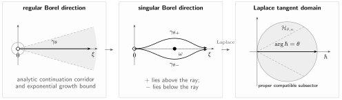
Directional data in the $\xi$-plane. A regular ray supports one Laplace contour. A singular point $\omega$ requires the lateral path $\gamma_{\theta+}$, displaced counterclockwise from the central ray, or $\gamma_{\theta-}$, displaced clockwise. When traversed outward, a small upper indentation is locally clockwise and a lower indentation is locally counterclockwise. Exponential growth of type $\kappa$ is overcome in the tangent domain $\operatorname{Re}(\ee^{\ii\theta}/\hbar)>\kappa$; the dashed rays in its final panel bound one proper compatible subsector.

Large-parameter notation reverses a familiar phase

Exact-WKB sources often use $\eta=1/\hbar$ and the kernel $\ee^{-\eta\xi}$. Then $\arg\eta=-\arg\hbar$. Never translate a source’s symbol $\theta$ by name alone; inspect the kernel and the actual Borel ray.

The alternating Euler series has an unobstructed sum

Consider

$$\widehat E_-(\hbar) := \sum_{n=0}^{\infty} (-1)^n n!\hbar^{n+1}.$$

It is Gevrey-1 and divergent for every $\hbar\neq0$. Its shifted Borel transform is nevertheless elementary:

$$\mathcal B\widehat E_-(\xi) = \sum_{n=0}^{\infty}(-\xi)^n = \frac{1}{1+\xi}.$$

The only finite singularity is at $\xi=-1$, so the positive ray is regular. For $\operatorname{Re}(1/\hbar)>0$,

$$\begin{aligned} E_-(\hbar) &:= \mathcal S_0\widehat E_-(\hbar) \\ &= \int_0^\infty \frac{\ee^{-\xi/\hbar}}{1+\xi} \,\dd\xi \\ &= \ee^{1/\hbar}E_1(1/\hbar), \end{aligned}$$

where the last expression uses the branch obtained from this integral. For positive $\hbar$, the Gevrey remainder is visible without invoking a general theorem. The finite geometric identity gives

$$\frac1{1+\xi} = \sum_{n=0}^{N-1}(-\xi)^n + (-1)^N\frac{\xi^N}{1+\xi},$$

and hence

$$\left| E_-(\hbar) - \sum_{n=0}^{N-1}(-1)^n n!\hbar^{n+1} \right| \leq N!\hbar^{N+1}.$$

The formal series satisfies the Euler equation coefficient by coefficient,

$$\hbar^2\widehat E_-' + \widehat E_- = \hbar.$$

Differentiation under the convergent integral proves that its Borel sum satisfies the same equation exactly:

$$\hbar^2 E_-' + E_- = \hbar.$$

This example separates two facts that are often conflated: the power series diverges, yet its Borel transform is regular in the desired direction and reconstructs a distinguished analytic solution.

A pole on the ray produces two lateral sums

Change only the coefficient signs:

$$\widehat E_+(\hbar) := \sum_{n=0}^{\infty}n!\hbar^{n+1}, \qquad \mathcal B\widehat E_+(\xi) = \frac1{1-\xi}.$$

Now the pole $\xi=1$ lies on the positive Borel ray. Define the lateral sums, whenever the limits exist, by

$$\mathcal S_{\theta+} := \lim_{\epsilon\downarrow0} \mathcal S_{\theta+\epsilon}, \qquad \mathcal S_{\theta-} := \lim_{\epsilon\downarrow0} \mathcal S_{\theta-\epsilon}.$$

The $+$ contour is counterclockwise from the central ray—above the positive real axis when $\theta=0$—and the $-$ contour is clockwise, or below. Fix the discontinuity convention

$$\operatorname{Disc}_\theta := \mathcal S_{\theta+} - \mathcal S_{\theta-}.$$

For positive $\hbar$, indentation of the pole gives

$$\begin{aligned} \mathcal S_{0+}\widehat E_+ &= \operatorname{PV} \int_0^\infty \frac{\ee^{-\xi/\hbar}}{1-\xi} \,\dd\xi + \pi\ii\ee^{-1/\hbar}, \\ \mathcal S_{0-}\widehat E_+ &= \operatorname{PV} \int_0^\infty \frac{\ee^{-\xi/\hbar}}{1-\xi} \,\dd\xi - \pi\ii\ee^{-1/\hbar}. \end{aligned}$$

Equivalently, the principal-value part is $\ee^{-1/\hbar}\operatorname{Ei}(1/\hbar)$. Subtraction yields the exact signed jump

$$\boxed{ \operatorname{Disc}_0\widehat E_+ = 2\pi\ii\ee^{-1/\hbar} }.$$

The sign follows from orientation. Upper-forward minus lower-forward closes clockwise around the pole. When this is the only obstruction enclosed between the two contours and the connecting pieces contribute no boundary term, a simple pole of the Borel transform at $\xi=A$ therefore gives

$$\operatorname{Disc}_\theta\widehat f = -2\pi\ii \operatorname{Res}_{\xi=A} \left[ \ee^{-\xi/\hbar} \mathcal B\widehat f(\xi) \right].$$

Here the residue is $-\ee^{-1/\hbar}$. Both lateral sums have the same Gevrey expansion because their difference is flat for $\operatorname{Re}(1/\hbar)>0$.

The formal and lateral functions obey

$$\hbar^2E_+' - E_+ = -\hbar.$$

Their difference solves the homogeneous equation, since

$$\hbar^2\partial_\hbar\ee^{-1/\hbar} - \ee^{-1/\hbar} =0.$$

This calculation establishes a lateral difference only. Page 2 will explain how singularities of continued Borel germs organize general Stokes discontinuities and when the stronger word resurgent applies.

An odd-power model for a quantum WKB correction

For $A>0$, consider the deliberately solvable formal model

$$\widehat W_A(\hbar) := \sum_{k=1}^{\infty} \frac{(2k-2)!}{A^{2k-1}} \hbar^{2k-1}.$$

Its parity matches a quantum-only Voros correction, but no claim is being made that it comes from a particular ODE. Its Borel transform is

$$\begin{aligned} \mathcal B\widehat W_A(\xi) &= \sum_{k=1}^{\infty} \frac{\xi^{2k-2}}{A^{2k-1}} \\ &= \frac{A}{A^2-\xi^2}. \end{aligned}$$

The two singularities $\xi=\pm A$ remember an action scale and its opposite. Since the residue at $\xi=A$ is $-1/2$,

$$\operatorname{Disc}_0\widehat W_A = \pi\ii\ee^{-A/\hbar}.$$

This is a model of the mechanism, not a universal exact-WKB jump formula. In an ODE, the singularity type and its coefficient depend on the normalized solution, continuation path, turning points and poles, and the Stokes chamber.

What is actually Borel transformed in WKB

Chapter 8 defined the formal quantum period of a declared closed or regularized cycle $\gamma$ by

$$\widehat\Pi_\gamma(\hbar) = \Pi_{\gamma,0} + \sum_{k=1}^{\infty} \Pi_{\gamma,2k}\hbar^{2k}.$$

Do not silently replace ℏ by ℏ²

If $\Pi_{\gamma,2k}$ has the common scale $\Gamma(2k+1)$, this period is Gevrey-1 as a series in $\hbar$. Reindexing it as a series in $t=\hbar^2$ makes the same coefficient scale Gevrey-2 in $t$, because

$$(2k)! = \frac{4^k}{\sqrt\pi} \Gamma\!\left(k+\frac12\right)k! \asymp \frac{4^k}{\sqrt{\pi k}}(k!)^2.$$

Here Gevrey-$s$ in $t$ means a coefficient bound of the form $C A^k(k!)^s$. The summability order changes with the chosen small variable.

The total formal exponent and its quantum-only correction are

$$\begin{aligned} \widehat V_\gamma^{\mathrm{tot}} &:= \frac{\widehat\Pi_\gamma}{\hbar} = \frac{\Pi_{\gamma,0}}{\hbar} + \widehat V_\gamma^{\mathrm q}, \\ \widehat V_\gamma^{\mathrm q} &:= \sum_{k=1}^{\infty} \Pi_{\gamma,2k}\hbar^{2k-1}. \end{aligned}$$

The classical transmonomial $\exp(\Pi_{\gamma,0}/\hbar)$ is not fed into the ordinary power-series Borel transform. It is declared and factored first. The two relevant Borel transforms are

$$\begin{aligned} \mathcal B \left( \widehat\Pi_\gamma-\Pi_{\gamma,0} \right) &= \sum_{k=1}^{\infty} \Pi_{\gamma,2k} \frac{\xi^{2k-1}}{(2k-1)!}, \\ \mathcal B\widehat V_\gamma^{\mathrm q} &= \sum_{k=1}^{\infty} \Pi_{\gamma,2k} \frac{\xi^{2k-2}}{(2k-2)!}. \end{aligned}$$

They differ by one Borel integration:

$$\mathcal B \left( \widehat\Pi_\gamma-\Pi_{\gamma,0} \right)(\xi) = \int_0^\xi \mathcal B\widehat V_\gamma^{\mathrm q}(\eta) \,\dd\eta.$$

If the quantum correction is summable in direction $\theta$ and the chosen summability class is closed under exponentiation, the sectorial Voros symbol of the oriented cycle $\gamma$ takes the form

$$\mathcal V_{\gamma,\theta} = \exp\!\left( \frac{\Pi_{\gamma,0}}{\hbar} \right) \exp\!\left( \mathcal S_\theta \widehat V_\gamma^{\mathrm q} \right).$$

This formula is conditional: the cycle or relative path, its orientation, and every regularization datum from Chapter 8 remain part of the object. Orientation already carries the sign:

$$\mathcal V_{-\gamma,\theta} = \mathcal V_{\gamma,\theta}^{-1}.$$

It must not be multiplied by a second, independent sheet sign.

For a local solution on a regular domain, restore the exact Chapter 8 decomposition before separating its classical exponential. With $\sigma\in\{+1,-1\}$ and $\lambda_0=p\,\dd z$,

$$\begin{aligned} \widehat\psi_\sigma(z,\hbar) &= C_\sigma(\hbar) P_{\mathrm{even}}(z,\hbar)^{-1/2} \exp\!\left[ \frac{\sigma}{\hbar} \int_{z_0}^{z} P_{\mathrm{even}}(\zeta,\hbar)\,\dd\zeta \right] \\ &= \exp\!\left[ \frac{\sigma}{\hbar} \int_{z_0}^{z}\lambda_0 \right] \widehat a_\sigma(z,\hbar), \end{aligned}$$

where

$$\begin{aligned} \widehat a_\sigma :={}& C_\sigma(\hbar) P_{\mathrm{even}}^{-1/2} \\ &\times \exp\!\left[ \frac{\sigma}{\hbar} \int_{z_0}^{z} \left( P_{\mathrm{even}}\,\dd\zeta - \lambda_0 \right) \right]. \end{aligned}$$

The unit normalization of Chapter 8 has $C_\sigma=1$ and no intrinsic power of $\hbar$. If another normalization contains $\hbar^\alpha$, fix a branch of $\log\hbar$ and factor that algebraic term alongside the classical exponential before applying this page’s ordinary transform to the remaining power-series amplitude. Exact-WKB sources also use shifted transforms adapted directly to the full WKB solution; those are equivalent only after translating the normalization and factorial shift.

The minimum WKB passport

For the geometric exact-WKB applications later in this book, a complete summability claim should record every applicable entry:

Datum	Why it matters
Phase of $\hbar$ and Borel direction $\theta$	Selects the decaying Laplace kernel and possible singular ray
Open regular spatial domain $D$, with estimates locally uniform on compact $K\Subset D$	Controls uniformity; turning points and poles cannot be crossed silently
Sheet or Riccati sign $\sigma$	Selects the classical exponential branch
Basepoint and continuation path, or oriented cycle $\gamma$	Fixes the action and its analytic continuation
Turning-point or pole normalization, when such endpoints are present	Fixes half-contours, subtraction terms, logarithm branches, and scales
Stokes graph and chamber, when a graph criterion or inter-region continuation is invoked	Determines whether the chosen continuation meets saddle connections or walls
Claimed status	Distinguishes a proved theorem, a conditional application, and a conjectural physical identification

Boundary conditions do not appear in this passport because they have not yet been imposed. They enter Stage C.

Conditional transfer from a formal WKB identity

Suppose a normalized amplitude solves the transformed ODE formally on an open regular domain $D$, with Gevrey-1 coefficient bounds and Borel continuation and growth estimates uniform on every compact $K\Subset D$ in direction $\theta$. Suppose also that every $\hbar$-dependent ODE coefficient is convergent or belongs to the same summability algebra, and that its chosen sum is the analytic coefficient in the ODE. If the relevant $z$-derivatives and convolutions are justified under the Laplace integral, the amplitude’s directional sum solves the normalized ODE exactly on $D$. Proving those hypotheses is the analytic theorem; coefficient matching alone is not.

Rigorous exact-WKB existence and uniqueness theorems provide such hypotheses for broad classes of second-order equations, but they remain local or directional statements with specified domains. Turning-point and Stokes-graph criteria are introduced later in this chapter rather than smuggled into the word “exact.”

Reproducible checks

The companion script verifies the normalization and sign ledger with exact algebra where possible and high-precision quadrature where an integral is essential. It checks:

• Borel–Laplace moments and the two Borel conventions;
• the alternating Euler integral, exponential integral, remainder bound, and differential equation;
• the nonalternating pole residue, lateral discontinuity, and homogeneous jump equation;
• the paired singularities and jump of the odd WKB-type model;
• the coefficientwise relation between a quantum period and its quantum-only Voros correction;
• the full complex convergence condition $\operatorname{Re}(\ee^{\ii\theta}/\hbar)>\kappa$.

Download the Borel–Laplace summation checker

Run it from the project root:

python3 public/code/advanced-ode/borel-laplace-summation-check.py

The script tests this page’s analytic calibration. It is not a numerical proof of Borel summability for an unspecified WKB problem.

Common pitfalls

Factorial growth is not a summability theorem. A Gevrey-1 bound produces a local Borel germ. It does not guarantee continuation along a desired ray or control at infinity.

A regular germ can meet a singular ray. Knowing many Taylor coefficients near $\xi=0$ does not show that the positive real axis is free of singularities. This is exactly the difference between the two Euler examples.

The Borel and Laplace normalizations come as a pair. The shifted transform used here has no $1/\hbar$ in its inverse. The unshifted transform includes that factor.

The Borel direction is not merely $\arg\hbar$. Their compatibility is the inequality $\operatorname{Re}(\ee^{\ii\theta}/\hbar)>\kappa$. Literature written in $\eta=1/\hbar$ can reverse the apparent phase label.

An action exponential is not an ordinary Taylor tail. Factor $\exp(\mathcal A/\hbar)$ and any chosen $\hbar^\alpha$ before applying the elementary Borel transform to the normalized amplitude.

The two lateral sums need not agree. They can share every formal coefficient and differ by an exponentially flat term. Always state which side is called $+$ and which discontinuity convention is used.

Summed does not mean quantized. A Borel-summed local WKB solution still lacks global continuation, a boundary condition, and a spectral equation.

Exercises

Exercise 1 · Calibrate both Borel conventions

For $n\geq1$, evaluate the shifted Borel–Laplace image of $\hbar^n$ along a ray $\arg\xi=\theta$. Repeat the calculation for the unshifted transform of $\hbar^n$, including its $1/\hbar$ prefactor. State the common convergence condition.

Solution

The shifted transform sends

$$\hbar^n \longmapsto \frac{\xi^{n-1}}{\Gamma(n)}.$$

Set $\xi=\ee^{\ii\theta}t$. If $\operatorname{Re}(\ee^{\ii\theta}/\hbar)>0$, the gamma integral gives

$$\begin{aligned} \int_0^{\ee^{\ii\theta}\infty} \ee^{-\xi/\hbar} \frac{\xi^{n-1}}{\Gamma(n)} \,\dd\xi &= \frac{\ee^{\ii n\theta}}{\Gamma(n)} \frac{\Gamma(n)}{ (\ee^{\ii\theta}/\hbar)^n } \\ &= \hbar^n. \end{aligned}$$

The unshifted transform sends $\hbar^n$ to $\xi^n/n!$. Therefore

$$\begin{aligned} \frac1\hbar \int_0^{\ee^{\ii\theta}\infty} \ee^{-\xi/\hbar} \frac{\xi^n}{n!} \,\dd\xi &= \frac1\hbar \frac{\ee^{\ii(n+1)\theta}}{n!} \frac{n!}{ (\ee^{\ii\theta}/\hbar)^{n+1} } \\ &= \hbar^n. \end{aligned}$$

The same decay condition appears in both calculations. For $n=0$, the shifted convention retains the constant outside the integral, whereas the unshifted convention integrates it.

Exercise 2 · Derive the alternating Euler remainder

Starting from the positive-ray integral for $E_-(\hbar)$ with $\hbar>0$, prove the factorial remainder bound on this page and derive $\hbar^2E_-'+E_-=\hbar$ without using the special-function formula.

Solution

Insert

$$\frac1{1+\xi} = \sum_{n=0}^{N-1}(-\xi)^n + (-1)^N\frac{\xi^N}{1+\xi}$$

into the integral. The gamma moments produce the first $N$ formal terms, while

$$R_N = (-1)^N \int_0^\infty \ee^{-\xi/\hbar} \frac{\xi^N}{1+\xi} \,\dd\xi.$$

Since $1/(1+\xi)\leq1$ on the positive ray,

$$|R_N| \leq \int_0^\infty \ee^{-\xi/\hbar}\xi^N\,\dd\xi = N!\hbar^{N+1}.$$

For the ODE, differentiate under the integral and use $\partial_\hbar\ee^{-\xi/\hbar} =(\xi/\hbar^2)\ee^{-\xi/\hbar}$. Then

$$\begin{aligned} \hbar^2E_-'+E_- &= \int_0^\infty \ee^{-\xi/\hbar} \frac{\xi+1}{1+\xi} \,\dd\xi \\ &= \int_0^\infty \ee^{-\xi/\hbar}\,\dd\xi = \hbar. \end{aligned}$$

Exercise 3 · Fix the sign of a lateral jump

Let $g(\xi)=1/(1-\xi)$ and $\hbar>0$. Parameterize small upper and lower semicircles from $1-\rho$ to $1+\rho$. Compute their difference, upper minus lower, and verify that it solves the homogeneous Euler equation.

Solution

Near $\xi=1$, the Laplace integrand has residue

$$\operatorname{Res}_{\xi=1} \frac{\ee^{-\xi/\hbar}}{1-\xi} = -\ee^{-1/\hbar}.$$

The upper path is parameterized by $\xi=1+\rho\ee^{\ii t}$ with $t$ decreasing from $\pi$ to $0$; it is clockwise and contributes $-\ii\pi$ times the residue. The lower path has $t$ increasing from $-\pi$ to $0$ and contributes $+\ii\pi$ times the residue. Thus

$$\mathcal S_{0+}\widehat E_+ - \mathcal S_{0-}\widehat E_+ = -2\pi\ii(-\ee^{-1/\hbar}) = 2\pi\ii\ee^{-1/\hbar}.$$

Finally,

$$\hbar^2 \partial_\hbar\ee^{-1/\hbar} = \ee^{-1/\hbar},$$

so the discontinuity satisfies $\hbar^2y'-y=0$.

Exercise 4 · Replace the pole by a branch point

Let $A\neq0$ and $\operatorname{Re}\beta>0$. Show that

$$\widehat F_{A,\beta}(\hbar) = \sum_{n=0}^{\infty} \frac{\Gamma(n+\beta)}{\Gamma(\beta)} A^n\hbar^{n+1}$$

has shifted Borel transform $(1-A\xi)^{-\beta}$. What extra data are needed to define lateral sums when $1/A$ lies on the chosen ray and $\beta\notin\mathbb Z$?

Solution

The coefficient of $\hbar^{n+1}$ is $\Gamma(n+\beta)A^n/\Gamma(\beta)$. Division by $\Gamma(n+1)=n!$ gives

$$\mathcal B\widehat F_{A,\beta}(\xi) = \sum_{n=0}^{\infty} \frac{(\beta)_n}{n!} (A\xi)^n = (1-A\xi)^{-\beta}.$$

For nonintegral $\beta$, $\xi=1/A$ is a branch point rather than a pole. Normalize the germ by $(1-A\xi)^{-\beta}=1$ at $\xi=0$ and specify the homotopy classes of continuation paths passing above and below $1/A$; those paths determine the two lateral branches. A drawn branch cut records this choice but is not additional invariant data.

Along either lateral continuation the germ is $O(|\xi|^{-\operatorname{Re}\beta})$ at infinity, so its exponential-growth condition is automatic in a compatible Laplace direction. The lateral sums remain the directional limits defined above. If they are rewritten as boundary-value integrals on a cut and $\operatorname{Re}\beta\geq1$, the contour-limit or finite-part prescription must be retained: the separate improper integrals are not locally integrable at $1/A$.

Exercise 5 · Audit a proposed WKB sum

Suppose someone writes

$$\psi(z,\hbar) = \mathcal S_0 \left[ \exp\!\left( \frac1\hbar\int^z\sqrt{R_0}\,\dd z \right) \widehat a(z,\hbar) \right]$$

and calls it “the exact solution.” Identify the missing conventions and rewrite the expression in a form compatible with this page.

Solution

The formula does not name a sheet of $\sqrt{R_0}$, a basepoint or continuation path, a spatial domain, a branch of any algebraic factor, or the side of the Borel ray if that ray is singular. It gives no Gevrey estimate, continuation theorem, exponential-growth bound, or uniformity in $z$. If a graph criterion or continuation between regions is invoked, it also omits the Stokes graph and chamber; if a turning point or pole is an endpoint, it omits the corresponding normalization. It supplies no boundary condition that would select a spectral solution.

After choosing a sign $\sigma$, a basepoint $z_0$, a path contained in a declared regular domain, and the relevant branches, restore the Chapter 8 amplitude:

$$\begin{aligned} \widehat a_\sigma :={}& C_\sigma P_{\mathrm{even}}^{-1/2} \\ &\times \exp\!\left[ \frac{\sigma}{\hbar} \int_{z_0}^{z} \left( P_{\mathrm{even}}\,\dd\zeta - \lambda_0 \right) \right]. \end{aligned}$$

If the amplitude satisfies the uniform summability passport in a regular direction $\theta$, its sectorial realization is

$$\psi_{\sigma,\theta} = \exp\!\left[ \frac{\sigma}{\hbar} \int_{z_0}^{z}\lambda_0 \right] \mathcal S_\theta \widehat a_\sigma(z,\hbar).$$

This is a normalized directional solution under the stated hypotheses—not yet a globally continued or spectrally quantized one. If $C_\sigma$ contains an explicit $\hbar^\alpha$, that factor is kept outside $\mathcal S_\theta$ after a branch of $\log\hbar$ is fixed.

References

• N. Nikolaev, “Existence and Uniqueness of Exact WKB Solutions for Second-Order Singularly Perturbed Linear ODEs,” Communications in Mathematical Physics 400 (2023), 463–517. Appendix A treats Gevrey asymptotics, Appendix C develops Borel–Laplace reconstruction, and Section 5 proves conditional exact-WKB existence, uniqueness, and summability results.
• T. Kawai and Y. Takei, Algebraic Analysis of Singular Perturbation Theory, Translations of Mathematical Monographs 227, AMS (2005). A standard exact-WKB reference with the analytic and microlocal framework.
• K. Iwaki and T. Nakanishi, “Exact WKB Analysis and Cluster Algebras,” Journal of Physics A 47 (2014), 474009; see Sections 2.3–2.8 and 3.1 for formal WKB solutions, normalizations, Borel sums, summability conditions, and Voros symbols.
• K. Iwaki, Les Houches Lectures on Exact WKB Analysis and Painlevé Equations (2025; revised 2026), Proposition 1.6 and Section 1.2.1. A concise modern bridge from WKB coefficient estimates to Borel transforms and Laplace integrals.
• W. Balser, From Divergent Power Series to Analytic Functions, Lecture Notes in Mathematics 1582, Springer (1994), Chapters 1–3.
• D. Sauzin, Introduction to 1-Summability and Resurgence (2014), especially the first part and the Euler-series examples.
• A. D. Sokal, “An Improvement of Watson’s Theorem on Borel Summability,” Journal of Mathematical Physics 21 (1980), 261–263. This gives the critical-opening Nevanlinna–Sokal refinement.
• G. N. Watson, “A Theory of Asymptotic Series,” Philosophical Transactions of the Royal Society A 211 (1912), 279–313.
• NIST Digital Library of Mathematical Functions, §2.4(i), “Watson’s Lemma.”
• D. Dorigoni, “An Introduction to Resurgence, Trans-Series and Alien Calculus,” Annals of Physics 409 (2019), 167914, Sections 2 and 4 for the Borel convention, Euler examples, and lateral sums.
• G. Nemes, “On the Borel Summability of WKB Solutions of Certain Schrödinger-Type Differential Equations,” Journal of Approximation Theory 265 (2021), 105562, for uniform WKB error bounds and summability on large spatial domains.

Page 2 studies the analytic continuation beyond the first Borel germ: resurgent singularities, their local data, and the discontinuities that relate directional sums. Only after that does Stage B introduce the quadratic differential and its spatial Stokes graph.