Stage B: Quadratic Differentials and Stokes Graphs

Page 2 described singularities and jumps in the Borel plane. Stage B now asks where the relevant action phases come from in the spatial variable. The answer begins with the leading quadratic differential, but it is not obtained by drawing arbitrary cuts between its turning points. A Borel direction rotates the differential, its horizontal critical trajectories form a phase-dependent skeleton, and the complementary regions organize compatible WKB normalizations.

The local geometry is exact: a simple zero has three critical prongs, a simple pole has one, and a pole of order $n\geq3$ has $n-2$ asymptotic directions. The global geometry is subtler. Critical leaves can join, close, spiral, or recur; an action with the right phase need not have a saddle trajectory representing it. Those distinctions are what keep a useful Stokes graph from becoming a misleading sketch.

This page constructs the graph and relates its orientation to WKB dominance. It does not yet write an Airy or simple-pole connection matrix, mutate a Voros symbol, or impose a boundary condition.

Page question

For a declared Borel direction, how does the quadratic differential determine the Stokes trajectories, their critical graph, and the parameter walls on which that graph changes?

Status ledger

Statement used on this page	Status
$\phi_\theta=\ee^{-2\ii\theta}\phi_0$	Exact translation of the book’s Borel–Laplace convention
Natural-coordinate foliation and sheet independence	Exact local geometry
Local prong and asymptotic-direction counts	Exact local classification
Leading dominance test	Leading WKB statement away from zeros and poles
Airy rays and Weber action	Exact classical calculations
A realized saddle connection has phase-aligned action	Necessary exact consequence
Every aligned period is represented by a saddle connection	False without an additional geometric existence argument
Finite strip decomposition	Theorem only under finite-type and no-recurrence hypotheses
Borel summability along complete WKB rays	Published theorem under the stated analytic, geometric, and uniformity hypotheses
A saddle-free graph is necessary for every local sum	False; it is a powerful sufficient criterion in standard frameworks
Connection multipliers, Voros mutations, and quantization	Deferred to Pages 4–6

The Borel angle selects the spatial foliation

Retain the spectral convention of Chapter 8,

$$\begin{aligned} -\hbar^2\psi''+V(z,\hbar)\psi &=E\psi, \\ \hbar^2\psi'' &=R(z,\hbar)\psi, \\ R(z,\hbar) &=R_0(z)+O(\hbar), \\ R_0 &=V_0-E. \end{aligned}$$

The leading quadratic differential on the base curve $C$ and its tautological square root on the normalized spectral cover $\pi:\widehat\Sigma\to C$ are

$$\begin{aligned} \phi_0 &=R_0(z)\,\dd z^2, & \lambda_0 &=y\,\dd z, \\ y^2 &=R_0(z), & \tau^*\lambda_0 &=-\lambda_0. \end{aligned}$$

Fix the book’s Borel half-ray

$$L_\theta=\ee^{\ii\theta}\mathbb R_+,$$

used with the Laplace kernel $\ee^{-\xi/\hbar}$. The phase selected on the base is

$$\phi_\theta = \ee^{-2\ii\theta}\phi_0.$$

On a chosen sheet and along a path from a finite critical point $a$, define

$$\begin{aligned} W_a(z) &= \int_a^z\lambda_0, \\ w_{\theta,a}(z) &= \ee^{-\ii\theta}W_a(z) = \int_a^z\sqrt{\phi_\theta}. \end{aligned}$$

This minus sign is part of the convention passport. Much of the exact-WKB literature uses the large parameter $\eta=1/\hbar$ and a direction $\alpha=\arg\eta$. A formula written there as $\phi_\alpha=\ee^{2\ii\alpha}\phi_0$ agrees with this page because

$$\alpha=-\theta, \qquad \ee^{2\ii\alpha}\phi_0 = \ee^{-2\ii\theta}\phi_0.$$

Copying the sign while silently replacing $\eta$ by $\hbar$ rotates every phase label the wrong way.

The angle $\theta$ labels the Borel contour and the graph. The actual phase $\vartheta=\arg\hbar$ is a separate datum: Laplace decay only requires $\cos(\theta-\vartheta)>0$, together with the growth bounds of Page 1. The cleanest geometric calibration uses the central ray $\vartheta=\theta$; off that ray, the graph angle and the exponential dominance angle should both remain visible.

Two periodicities already differ:

$$\phi_{\theta+\pi}=\phi_\theta, \qquad w_{\theta+\pi,a}=-w_{\theta,a}.$$

Thus the unoriented graph is $\pi$-periodic, while an oriented Borel half-ray, a sheet label, and a dominance label are $2\pi$-periodic. The graph depends on $R_0$ rather than on all of $R(z,\hbar)$. Subleading coefficients still matter to transport amplitudes, summability estimates, pole normalizations, and connection constants.

Natural coordinates separate Stokes curves from equal magnitude

At an ordinary point, a regular parametrized curve $z=\gamma(s)$ is horizontal for $\phi_\theta$ when

$$\ee^{-2\ii\theta} R_0(\gamma(s))\dot\gamma(s)^2 \in\mathbb R_{>0}.$$

On a chosen square-root sheet this is equivalent to

$$\operatorname{Im} \left[ \ee^{-\ii\theta} y(\gamma(s))\dot\gamma(s) \right] =0.$$

Consequently, every regular horizontal leaf becomes a straight line in the natural coordinate:

$$\operatorname{Im}w_{\theta,a} = \text{constant}.$$

With positive natural-length orientation one may integrate

$$\frac{\dd z}{\dd s} = \frac{\ee^{\ii\theta}}{y(z)}, \qquad \frac{\dd w_{\theta,a}}{\dd s}=1.$$

The deck transformation sends $y$ and $w_{\theta,a}$ to their negatives. It reverses this orientation and exchanges the labels $+$ and $-$, but it leaves the unoriented base foliation unchanged. The condition is also coordinate invariant: under $z=z(u)$, the coefficient becomes $R_0(z(u))(\dd z/\dd u)^2$, exactly as a quadratic differential must.

The vertical foliation is different:

$$\operatorname{Re}w_{\theta,a} = \text{constant}, \qquad \phi_\theta(\dot\gamma,\dot\gamma) \in\mathbb R_{<0}.$$

Why does this distinction matter? Away from the divisor, the leading WKB branches have the form

$$\psi_\pm(z,\hbar) \sim R_0(z)^{-1/4} \exp\left[ \pm\frac{W_a(z)}{\hbar} \right].$$

For $\hbar=|\hbar|\ee^{\ii\vartheta}$,

$$\log\left| \frac{\psi_+}{\psi_-} \right| \sim \frac{2}{|\hbar|} \operatorname{Re} \left[ \ee^{-\ii\vartheta}W_a(z) \right].$$

On the central ray $\vartheta=\theta$, the horizontal critical curve from $a$ has $\operatorname{Im}w_{\theta,a}=0$; along an oriented lift, one exponential grows while the other decays. The two leading exponentials instead have equal magnitude on

$$\operatorname{Re}w_{\theta,a}=0,$$

the vertical leaf through $a$. Crossing a horizontal Stokes curve does not in general exchange dominance, and an equal-magnitude leaf may run through the interior of a Stokes region.

Names vary; equations travel safely

Parts of the physics literature exchange the terms Stokes and anti-Stokes. This book calls the horizontal critical leaves $\operatorname{Im}w_{\theta,a}=0$ Stokes curves and calls the vertical leaves $\operatorname{Re}w_{\theta,a}=0$ equal-magnitude curves. Translate a source by these equations, not by its nouns.

The divisor order fixes the local trajectory atlas

Let $x=z-z_0$ and suppose

$$\phi_0 = a x^m\left(1+O(x)\right)\dd x^2, \qquad a\neq0.$$

For $m\neq-2$, integration gives the leading natural coordinate

$$w_\theta(x) \sim \frac{2\ee^{-\ii\theta}\sqrt a}{m+2} x^{(m+2)/2}.$$

At a zero of order $m\geq1$, or at a simple pole $m=-1$, a horizontal critical trajectory has $\arg w_\theta\in\pi\mathbb Z$. Its possible tangent directions are therefore

$$\arg x = \frac{ 2\theta-\arg a+2\pi k }{m+2}.$$

For a zero, $k=0,\ldots,m+1$ gives $m+2$ distinct half-trajectories. For a simple pole, there is one. The vertical prongs follow by replacing $\theta$ with $\theta+\pi/2$.

Point of $\phi_0$	Quadratic-metric distance	Horizontal local behavior
Zero of order $m\geq1$	Finite	$m+2$ prongs, spaced by $2\pi/(m+2)$
Simple zero	Finite	Three prongs
Double zero	Finite	Four prongs; not an Airy point
Simple pole	Finite	One prong on the base
Double pole	Infinite	Radial, circular, or spiral leaves
Pole of order $n\geq3$	Infinite	$n-2$ distinguished asymptotic directions

The distance claim follows from the radial test

$$\int_0^\varepsilon r^{m/2}\,\dd r<\infty \quad\Longleftrightarrow\quad m>-2.$$

A simple pole deserves special care. With $x=t^2$ on the normalized cover, its leading square root satisfies

$$\lambda_0 \sim \sqrt a\,x^{-1/2}\dd x = 2\sqrt a\,\dd t.$$

The lifted one-form is regular and nonzero; the one-prong base picture comes from ramification. Chapter 8 therefore called this a simple-pole branch point. Some exact-WKB sources call the same point a turning point of simple-pole type. Its connection multiplier is not the ordinary Airy multiplier and belongs on Page 4.

For a pole of order $n\geq3$,

$$\phi_0 = a x^{-n}\left(1+O(x)\right)\dd x^2,$$

the $n-2$ distinguished asymptotic directions are

$$\begin{gathered} \arg x = \frac{ \arg a-2\theta+2\pi j }{n-2}, \\ j=0,\ldots,n-3. \end{gathered}$$

These are limiting tangent directions at an infinite-distance point, not finite-valence prongs in the same metric sense as those at a zero.

Double poles are controlled by a residue

At a double pole, choose one sheet and use the residue convention of Chapter 8. After an adapted holomorphic change of local coordinate, one may write

$$\begin{aligned} \lambda_0 &= \rho\frac{\dd x}{x}, \\ w_\theta &= \rho_\theta\Log x, \\ \rho_\theta &= \ee^{-\ii\theta}\rho. \end{aligned}$$

Write $\rho_\theta=u+\ii v$ and $x=r\ee^{\ii\alpha}$. Horizontal leaves satisfy

$$v\log r+u\alpha = \text{constant}.$$

Hence, in this adapted coordinate, they are radial when $\rho_\theta$ is real, circular when it is purely imaginary, and logarithmic spirals in the generic case. Some texts multiply the residue of the quadratic differential by an extra factor of $\ii$; their real and imaginary cases then appear reversed. The invariant datum here is the explicitly displayed residue of $\lambda_0$.

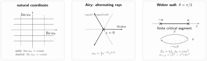
Three calibrations of the convention. Left: horizontal leaves of $\phi_\theta$ are solid and the vertical foliation is dashed; only its zero-level leaf through the chosen action basepoint is an equal-magnitude curve. Center: at $\theta=0$, Airy’s three Stokes rays alternate with three equal-magnitude rays. Right: at the Weber wall $\theta=\pi/2$, the real interval between the two turning points is a finite horizontal trajectory. For the chosen lift $\beta$, let $\delta=\beta-\tau_*\beta$ and $A=\int_\beta\lambda_0$; then $Z_\delta=2A$. The Weber panel isolates this critical segment and is not a drawing of the complete global graph.

A Stokes graph is a critical skeleton, not a branch-cut diagram

It is useful to separate three parts of the divisor:

$$\begin{aligned} P_0 &=\{\text{zeros of }\phi_0\}, \\ P_s &=\{\text{simple poles of }\phi_0\}, \\ P_\infty &=\{\text{poles of order at least two}\}. \end{aligned}$$

The points in $P_0\cup P_s$ are finite critical points in the metric of $\phi_\theta$; those in $P_\infty$ are infinite critical points. For a fixed phase $\theta$:

• A Stokes curve is a critical horizontal trajectory with an endpoint in $P_0\cup P_s$.
• The Stokes graph $G_\theta$ is the union of the declared critical points and their Stokes curves.
• A Stokes region is a connected component of $C\setminus G_\theta$.
• A Stokes segment or saddle trajectory has finite critical points at both ends, possibly the same point.
• The graph is saddle-free when it has no Stokes segment. It still contains Stokes curves.

Branch cuts used to draw the two sheets of $\widehat\Sigma$ are not edges of $G_\theta$. Moving such a cut changes a presentation of the cover. Rotating $\theta$ generally changes the actual trajectory foliation.

Globally, maximal horizontal trajectories have the following behaviors.

Trajectory type	Forward and backward behavior
Saddle	Both ends approach finite critical points
Separating	One end is finite and the other is an infinite critical point
Generic	Both ends approach infinite critical points
Closed	A periodic simple closed leaf in a ring domain
Recurrent	Nonclosed, with a nontrivial recurrent limit set

A ring domain is a maximal annulus swept out by closed leaves. A degenerate ring domain has a double pole as one collapsed boundary component. Spiral domains can occur when recurrent behavior is allowed. The older phrase divergent trajectory sometimes means a nonclosed leaf with a multi-point limit set; it should not be confused with an ordinary generic leaf that tends to a pole.

Without a no-recurrence or comparable finite-type hypothesis, the critical skeleton need not be a finite CW graph. For a saddle-free GMN differential in the sense of Bridgeland–Smith—on a compact surface, with simple zeros and at least one pole of order at least two—closed and recurrent trajectories are absent. Removing the critical points and the finitely many separating trajectories then decomposes the surface into natural-coordinate pieces:

$$\begin{aligned} \text{horizontal strip:} &\quad a<\operatorname{Im}w_\theta<b, \\ \text{half-plane:} &\quad \operatorname{Im}w_\theta>0, \end{aligned}$$

up to translations and reflections of $w_\theta$. The generic leaves in a strip run between infinite critical points; those in a half-plane approach the same higher-order pole at both ends. Simple poles may occur on strip boundaries. If a phase-adjusted double-pole residue is purely imaginary in this page’s $\operatorname{Res}\lambda_0$ convention, the circular foliation lies in a degenerate ring domain whose other boundary contains saddle trajectories; it is therefore outside this saddle-free conclusion. These hypotheses must be declared before finite graph combinatorics is used.

Stokes regions and Stokes chambers live in different spaces

A Stokes region is a subset of the $z$-surface for fixed parameters and fixed $\theta$. A Stokes chamber is a subset of the external space of energies, couplings, and phase. Its walls include loci where a saddle trajectory is realized; its boundary can also meet a discriminant, where zeros or poles collide and the divisor type itself changes.

Object	Lives in	Changes when
Stokes curve	The base curve $C$	The horizontal critical leaf moves
Stokes region	$C\setminus G_\theta$	Its critical boundary reconnects
Stokes wall	Parameter–phase space	A saddle trajectory is realized
Discriminant	Parameter space	The divisor or local turning-point type changes
Stokes chamber	Complement of the excluded walls	The graph’s finite-type isotopy class is locally constant

For an actual saddle connection $\ell$ from $a$ to $b$, choose a sheet and orientation and set

$$A_\ell = \int_\ell\lambda_0.$$

Because the trajectory is horizontal,

$$\operatorname{Im} \left( \ee^{-\ii\theta}A_\ell \right)=0, \qquad \theta=\arg A_\ell\pmod\pi.$$

If $\ell$ joins two branch points, its standard doubled lift is a closed saddle class $\gamma$ with a compatible orientation and

$$Z_\gamma := \oint_\gamma\lambda_0 = 2A_\ell.$$

Three normalizations should therefore not be collapsed:

Geometric object	Classical action entering it
One-sheet natural coordinate from $a$	$W_a(z)=\int_a^z\lambda_0$
Ratio of the two WKB exponentials	$2W_a(z)/\hbar$
Closed lift of a branch-to-branch saddle	$Z_\gamma=2A_\ell$ in the stated orientation

The factor of two does not alter the wall phase, but it changes the location assigned to a Borel singularity. Moreover, phase alignment is only necessary. An arbitrary class with $\operatorname{Im}(\ee^{-\ii\theta}Z_\gamma)=0$ need not possess a horizontal geodesic representative. A wall is the locus of geometric existence of the saddle, not merely the vanishing of one imaginary part.

At an isolated regular wall, the graphs at $\theta-\varepsilon$ and $\theta+\varepsilon$ are the two saddle reductions. Their elementary reconnection is called a flip. A loop saddle around a double pole leads to a pop, and simple-pole segments have their own mutation rules. This page records the geometry; Page 5 will act on Voros symbols.

Airy calibrates three Stokes rays and three other rays

For

$$\left[-\hbar^2\partial_z^2+z\right]\psi=0,$$

one has

$$\begin{aligned} R_0 &=z, \\ W_0(z) &=\frac23z^{3/2}, \\ w_{\theta,0}(z) &= \frac23\ee^{-\ii\theta}z^{3/2}. \end{aligned}$$

The three horizontal Stokes rays from the simple zero are

$$\arg z = \frac{2\theta}{3} + \frac{2\pi k}{3}, \qquad k=0,1,2.$$

The three vertical equal-magnitude rays interlace them:

$$\arg z = \frac{2\theta+(2k+1)\pi}{3}, \qquad k=0,1,2.$$

At $\theta=0$, the Stokes rays have arguments $0,2\pi/3,4\pi/3$, while the equal-magnitude rays have arguments $\pi/3,\pi,5\pi/3$. Along the positive real axis with $\hbar>0$,

$$\psi_- \sim z^{-1/4} \exp\left( -\frac{2z^{3/2}}{3\hbar} \right)$$

is subdominant and matches the decaying Airy branch up to normalization. Along the negative real axis the two leading exponentials have equal magnitude and are oscillatory.

Infinity supplies an independent global check. With $x=1/z$,

$$z\,\dd z^2 = x^{-5}\,\dd x^2.$$

The order-five pole has $5-2=3$ asymptotic directions, precisely the three endpoints at infinity of the Airy Stokes curves. There is no finite saddle segment, so the Airy graph is saddle-free.

Weber exhibits a genuine graph wall

Take the same Weber convention as Chapter 8,

$$\left[-\hbar^2\partial_z^2+z^2\right]\psi = a^2\psi, \qquad a>0,$$

so

$$R_0=z^2-a^2.$$

On the sheet above $-a<x<a$ with

$$y(x)=\ii\sqrt{a^2-x^2},$$

the open turning-point action and its standard doubled lift are

$$\begin{aligned} A &= \int_{-a}^{a}\lambda_0 = \ii\int_{-a}^{a} \sqrt{a^2-x^2}\,\dd x = \frac{\ii\pi a^2}{2}, \\ Z_\delta &= \oint_\delta\lambda_0 = 2A = \ii\pi a^2. \end{aligned}$$

At $\theta=0$, the real classically allowed interval is pointwise vertical because

$$R_0(x)=x^2-a^2<0 \qquad(-a<x<a).$$

Equivalently, every partial action from $-a$ to an interior point is purely imaginary. The interval is therefore an equal-magnitude trajectory, not a Stokes segment in this book’s vocabulary. The horizontal wall occurs when

$$\operatorname{Im} \left( \ee^{-\ii\theta}A \right)=0,$$

namely

$$\theta=\frac\pi2\pmod\pi.$$

Direct substitution makes the geometry transparent:

$$\phi_{\pi/2} = -\left(z^2-a^2\right)\dd z^2 = \left(a^2-z^2\right)\dd z^2.$$

It is positive on $[-a,a]$, so that interval is an actual zero-to-zero Stokes segment. The graphs at $\pi/2-\varepsilon$ and $\pi/2+\varepsilon$ give its two saddle reductions. A presentation based on $p^2=E-V$ instead of $y^2=V-E$ looks rotated by $\pi/2$ because the corresponding WKB exponent contains an extra factor of $\ii$.

A reproducible graph-construction workflow

For a meromorphic problem with declared parameters, the following workflow keeps the exact deductions separate from numerical evidence.

1. Compactify the base. Transform the quadratic differential at infinity; do not infer its order from $R_0$ as a function alone.
2. Build the divisor passport. Record every zero and pole with its multiplicity, and distinguish finite from infinite critical points.
3. Declare the phase. State the Borel ray $L_\theta$, form $\phi_\theta$, and separately record the compatible sector of $\hbar$.
4. Seed the exact local directions. At a distance $\varepsilon$ from every finite critical point, use the analytic prong formula rather than a visual guess.
5. Track a square-root sheet. Integrate $\dd z/\dd s=\pm\ee^{\ii\theta}/y(z)$ with continuous branch tracking. Restarting a principal square root independently at each step can manufacture false turns.
6. Classify every endpoint. Stop at a finite critical point, a declared pole neighborhood, or a controlled escape boundary. Test for closed or recurrent behavior before treating the result as a finite graph.
7. Audit finite candidates by actions. Compute $A_\ell$ independently and test its phase. A plotted near-hit is not a proof of a saddle connection.
8. Scan both sides of a wall. Compare $G_{\theta-\varepsilon}$ and $G_{\theta+\varepsilon}$ while keeping the divisor fixed. A collision of critical points is a discriminant event, not a graph flip.
9. Record tolerances and topology. Save step-size, endpoint, and phase tolerances, and distinguish a numerically suggested isotopy class from a certified one.

The natural-coordinate ODE provides a useful invariant during integration:

$$\frac{\dd}{\dd s} w_{\theta,a}(z(s)) = \pm1.$$

Deviation of its imaginary part is therefore a direct trajectory error monitor.

What geometry proves about Borel summation

The graph is analytic input, not a self-sufficient summability proof. A precise published result can be stated in trajectory form. Consider

$$\hbar^2\psi'' + \hbar p(z,\hbar)\psi' + q(z,\hbar)\psi =0,$$

and put

$$D_0=p_0^2-4q_0.$$

Let $p$ and $q$ be holomorphic on $X\times S$, where $S$ is a sectorial domain whose opening arc $\mathcal A$ has angular width $\pi\leq|\mathcal A|\leq2\pi$, and assume that they admit locally uniform Gevrey asymptotic expansions along the closed arc $\mathcal A$. Fix a direction $\theta$ in the associated copolar arc of compatible Laplace directions, a sign $\alpha$, a regular normalization point $z_0$, a branch of $\sqrt{D_0}$ there, and a simply connected turning-point-free domain $U$ containing $z_0$. Suppose every WKB $(\theta,\alpha)$-ray from $U$ is complete.

For every $z\in U$, require a neighborhood $V\subset U$ and $R\gg1$ such that, on the corresponding remote ray domain $V_{\theta,\alpha,R}$, the logarithmic-derivative expression

$$\frac{1}{\sqrt{D_0}} \partial_z\log\sqrt{D_0},$$

is bounded and $p/\sqrt{D_0}$ and $q/D_0$ have the uniform asymptotics required in Theorem 5.1. Then Theorem 5.3 identifies the normalized formal WKB solution with its locally uniform Borel sum in direction $\theta$, on a possibly smaller Borel disk.

For Schrödinger form, $p=0$, $q=-R$, and

$$D_0=4R_0,$$

so the factor $4$ does not change the trajectories. Polynomial $\hbar$-dependence simplifies the coefficient hypotheses, but it does not remove completeness or the geometric bounds at poles. Published corollaries also cover suitable generic strip domains and closed trajectories in ring domains. Thus the absence of every saddle in the global graph is not necessary for every local WKB sum.

The classical graph criterion is still extremely effective. In the Iwaki–Nakanishi compact meromorphic framework—simple zeros, poles of order at least two, their stated subleading-potential conditions, admissible normalizations, and no saddle trajectory—a normalized WKB solution is Borel summable in each Stokes region. In the no-simple-pole setting, Corollary 2.21 also imposes the endpoint and relative-homology conditions of Lemma 2.20, in addition to avoidance of saddle trajectories. In the simple-pole extension, Theorem 2.10 assumes its Assumptions 2.3 and 2.7 and a path in the complement of zeros and simple poles that avoids every Stokes segment. Thus pathwise admissibility weakens global saddle freedom, but it does not replace the remaining analytic and endpoint hypotheses.

Provenance of the blanket graph statement

The 2014 exact-WKB paper attributes the analytic theorem behind its broad saddle-free graph criterion to unpublished work of Koike–Schäfke. Nikolaev’s 2023 peer-reviewed theorem proves the trajectory-local existence, uniqueness, and summability result under its own explicit hypotheses, but it should not be cited as a literal proof of every older global-path formulation. This page uses the published trajectory theorem as its rigorous core and records the classical graph criterion with its source framework.

Neither theorem says that the graph alone determines every Borel singularity or its local minor. In particular, the graph by itself does not determine

• a Stokes constant or connection multiplier;
• the special multiplier at a simple pole;
• every later-sheet Borel singularity;
• a global monodromy matrix;
• a boundary condition or a spectrum.

From a spatial edge to Page 4’s connection passport

Stage A and Stage B use related but differently oriented objects.

Datum	Periodicity or sign	Role
Unoriented graph $G_\theta$	$\theta$ modulo $\pi$	Spatial decomposition
Oriented Borel ray $L_\theta$	$\theta$ modulo $2\pi$	Laplace contour and lateral side
One-sheet action $A_\ell$	Changes sign under sheet exchange	Natural-coordinate length
Closed saddle period $Z_\gamma$	Changes sign under cycle reversal	Candidate Borel action scale
Actual phase $\arg\hbar$	Must lie in a compatible Laplace sector	Exponential dominance

A spatial saddle fixes an action phase, but only an orientation and a sheet decide whether $+Z_\gamma$ or $-Z_\gamma$ lies on the chosen Borel half-ray. Page 2’s local Borel singularity data then require analytic continuation and growth information beyond this geometric phase test.

Before applying any local connection formula on Page 4, record the following passport:

1. the Borel direction $\theta$ and the actual compatible $\hbar$-sector;
2. the sheet of $\lambda_0$ and the labels of $\psi_\pm$;
3. the normalization point or endpoint subtraction;
4. the oriented Stokes edge and its finite endpoint type;
5. the adjacent Stokes regions, ordered counterclockwise from the finite endpoint;
6. the sign of $\operatorname{Re}(\ee^{-\ii\vartheta}W_a)$ for the chosen actual phase $\vartheta=\arg\hbar$, reducing to $\operatorname{Re}w_{\theta,a}$ only on the central ray $\vartheta=\theta$;
7. the branch-cut presentation used to lift paths, without treating the cuts as graph edges;
8. whether the graph is saddle-free or only the chosen path is admissible.

These data determine which local solution is dominant and which triangular connection pattern is possible. The numerical multiplier itself is the next page’s calculation.

Reproducible checks

The Stokes-graph geometry checker verifies, with exact symbolic and numerical identities,

• the local prong-angle formula and its $\pi$-periodicity;
• the alternating Airy horizontal and equal-magnitude rays;
• the $n-2$ higher-pole count and polynomial behavior at infinity;
• the radial, circular, and spiral double-pole level sets;
• invariance of the trajectory equation under a coordinate change;
• the Weber open action, doubled closed action, and wall phase.

The checker deliberately does not infer that an aligned homology class has a saddle representative, prove Borel summability, or compute a connection coefficient. Those are geometric and analytic questions, not consequences of a finite symbolic identity test.

Common pitfalls

Copying a large-parameter phase without translation. If a source uses $\eta=1/\hbar$, then $\arg\eta=-\arg\hbar$. Translate the Borel ray and the phased differential together.

Calling the equal-magnitude locus a Stokes curve without declaring the convention. On this page, Stokes curves are horizontal and obey $\operatorname{Im}w_\theta=0$ at a critical endpoint. Equal magnitude means $\operatorname{Re}w_\theta=0$.

Treating a branch cut as a graph edge. A branch cut is a movable device for drawing the spectral cover. A Stokes edge is an intrinsic critical trajectory of the phased quadratic differential.

Reading saddle-free as curve-free. A saddle-free graph normally contains many separating Stokes curves. It contains no finite critical-to-critical Stokes segment.

Turning a necessary period test into a proof. An actual saddle has aligned action. An aligned abstract cycle need not have a horizontal geodesic representative.

Applying Airy at every branch point. A higher-order zero has more than three prongs, and a simple-pole branch point has one. Their local connection problems are not the ordinary simple-zero Airy problem.

Forgetting infinity. A polynomial $R_0$ of degree $d$ gives a pole of order $d+4$ for $R_0(z)\dd z^2$ at infinity and hence $d+2$ asymptotic directions.

Equating a spatial region with a parameter chamber. A Stokes region is a face on the $z$-surface. A chamber is a region in parameter–phase space over which the graph topology remains stable.

Exercises

1. Derive every finite critical prong

Let $\phi_0=a x^m(1+O(x))\dd x^2$ with $m\geq1$ or $m=-1$. Derive the horizontal and vertical tangent directions at $x=0$ and show that changing the square-root sheet does not change their unoriented set.

Solution

The leading natural coordinate is

$$w_\theta \sim \frac{2\ee^{-\ii\theta}\sqrt a}{m+2} x^{(m+2)/2}.$$

Horizontal critical leaves require $\arg w_\theta=k\pi$, so

$$\arg x = \frac{2\theta-\arg a+2\pi k}{m+2}.$$

For $m\geq1$, the values $k=0,\ldots,m+1$ are distinct modulo $2\pi$, giving $m+2$ prongs. When $m=-1$, there is one. Vertical leaves require $\arg w_\theta=\pi/2+k\pi$, hence

$$\arg x = \frac{2\theta+\pi-\arg a+2\pi k}{m+2}.$$

Changing sheets adds $\pi$ to $\arg\sqrt a$, which shifts $k$ by one. It permutes the same unoriented prongs and reverses their lifted orientation.

2. Rotate the Airy fan

For $\phi_0=z\,\dd z^2$, draw the horizontal and vertical rays at an arbitrary phase $\theta$. Verify that the two fans alternate and that $G_{\theta+\pi}=G_\theta$ as an unoriented graph.

Solution

Since $w_\theta=(2/3)\ee^{-\ii\theta}z^{3/2}$, horizontality gives

$$\arg z = \frac{2\theta}{3}+\frac{2\pi k}{3},$$

while verticality gives

$$\arg z = \frac{2\theta+(2k+1)\pi}{3}.$$

The second set is shifted by $\pi/3$, so the six rays alternate. When $\theta$ increases by $\pi$, the horizontal set shifts by $2\pi/3$, which merely permutes its three members. The oriented natural coordinate changes sign, so the full oriented data have not returned.

3. Classify a double-pole neighborhood

Let $\lambda_0\sim\rho\,\dd x/x$. Starting from $\operatorname{Im}(\ee^{-\ii\theta}\rho\Log x)=C$, classify the horizontal leaves and show that the sheet change leaves their base sets invariant.

Solution

Put $\ee^{-\ii\theta}\rho=u+\ii v$ and $x=r\ee^{\ii\alpha}$. The level equation is

$$v\log r+u\alpha=C.$$

If $v=0$, then $\alpha$ is constant and the leaves are radial. If $u=0$, then $r$ is constant and they are circles. If $uv\neq0$, then $\alpha=C/u-(v/u)\log r$, a logarithmic spiral. Sheet exchange sends $(u,v,C)$ to $(-u,-v,-C)$ and therefore leaves the same subsets of the base.

4. Prove coordinate invariance of the line field

Let $z=z(u)$ be biholomorphic and set $\widetilde R_0(u)=R_0(z(u))z'(u)^2$. Show that the horizontal trajectory equation in $u$ maps to the one in $z$.

Solution

For a path $u=u(s)$, its image satisfies $\dot z=z'(u)\dot u$. Hence

$$\ee^{-2\ii\theta} \widetilde R_0(u)\dot u^2 = \ee^{-2\ii\theta} R_0(z)\dot z^2.$$

One side is positive real exactly when the other is. Equivalently, $\sqrt{\widetilde R_0}\,\dd u=\sqrt{R_0}\,\dd z$ after a consistent sheet choice, so the natural coordinate itself is unchanged up to an additive constant and an overall sign.

5. Locate the Weber wall without a plot

For $R_0=z^2-a^2$ with $a>0$, compute the action across the real turning-point interval on the sheet $y=\ii\sqrt{a^2-x^2}$. Determine its horizontal phase and explain what the interval represents at $\theta=0$.

Solution

The area of a semicircle gives

$$A = \ii\int_{-a}^{a}\sqrt{a^2-x^2}\,\dd x = \frac{\ii\pi a^2}{2}.$$

Every partial action is purely imaginary because $R_0(x)=x^2-a^2<0$ in the open interval. Thus the interval is vertical at $\theta=0$. The total action satisfies $\operatorname{Im}(\ee^{-\ii\theta}A)=0$ when $\theta=\pi/2\pmod\pi$. At that phase, $\phi_\theta=(a^2-z^2)\dd z^2$ is positive on the interval, so the interval is a horizontal saddle connection. The closed lifted action is $2A=\ii\pi a^2$ in the stated orientation.

6. Audit the converse wall test

Suppose a homology class $\gamma$ satisfies $\operatorname{Im}(\ee^{-\ii\theta}Z_\gamma)=0$. Does this prove that $G_\theta$ has a saddle connection of class $\gamma$? What additional fact is missing?

Solution

No. The equation constrains only the integral of $\lambda_0$ over an abstract class. A saddle connection is a particular horizontal geodesic whose endpoints are finite critical points and whose interior contains no critical point. One must prove that such a geodesic representative exists with the required endpoints and topology. The period test is necessary after the trajectory is known, not sufficient before it is found.

7. Test two overstatements about summability

Assess the claims “a saddle connection makes every WKB solution nonsummable” and “a saddle-free graph proves summability without any further assumptions.”

Solution

Both are false. A saddle elsewhere need not obstruct a normalized solution supported on a complete admissible family of WKB rays, and published results also cover suitable closed trajectories in ring domains. Conversely, graph topology alone does not supply Gevrey bounds, coefficient control, completeness, pole estimates, or an admissible normalization. Saddle freedom is a strong sufficient geometric condition only inside a theorem whose analytic hypotheses are also satisfied.

References

• Nikolaev, N., “Existence and Uniqueness of Exact WKB Solutions for Second-Order Singularly Perturbed Linear ODEs”, Communications in Mathematical Physics 400 (2023), 463–517, §§4.3–4.5, Theorems 5.1 and 5.3, and Corollaries 5.2, 5.4, and 5.6. Gives the phased trajectories and the published trajectory-local existence, uniqueness, and Borel-summability theorem used here.
• Iwaki, K., and Nakanishi, T., “Exact WKB Analysis and Cluster Algebras”, Journal of Physics A 47 (2014), 474009, §§2.6–2.9 and §§3.2–3.3. Defines the phase-rotated graph, Stokes regions, saddle reductions, and the classical saddle-free summability framework in the $\eta=1/\hbar$ convention.
• Iwaki, K., and Nakanishi, T., “Exact WKB Analysis and Cluster Algebras II”, International Mathematics Research Notices 2016, 4375–4417, §§2.1–2.4. Extends the graph and summability framework to simple-pole branch points under additional coefficient hypotheses.
• Bridgeland, T., and Smith, I., “Quadratic Differentials as Stability Conditions”, Publications Mathématiques de l’IHÉS 121 (2015), 155–278, §§3.1–3.5. Supplies the local models, global trajectory taxonomy, finite-length trajectories, strip decomposition, and saddle-free finite-type geometry.
• Strebel, K., Quadratic Differentials, Springer, 1984, especially §§6 and 9–11. Standard reference for local critical-point geometry and global strip and ring domains.
• Koike, T., “On the Exact WKB Analysis of Second Order Linear Ordinary Differential Equations with Simple Poles”, Publications of the Research Institute for Mathematical Sciences 36 (2000), 297–319. Establishes the special local exact-WKB treatment required at simple poles.
• Nikolaev, N., “Geometry and Resurgence of WKB Solutions of Schrödinger Equations”, preprint, 2024, especially Theorem 4.1 and Propositions 4.3–4.6. Gives a modern geometric Borel dictionary under its stated global marked-curve and pole-control assumptions; cited here as a preprint.