Matone-Type and Accessory-Parameter Relations

Page 6 defined the quantum mirror map by an A-period. That construction answers a horizontal question on the Coulomb fibration: which operator modulus $u$ corresponds to a prescribed flat coordinate $a$? A Matone-type relation answers a different question: what does a derivative with respect to the ultraviolet coupling insert? An accessory-parameter relation asks a third: which coefficient of a normalized scalar oper is produced by that derivative?

These questions happen to meet in important rank-one examples, but the meeting is not automatic. The expectation value of a chiral operator, the curve coordinate $u$, the printed energy $E_{\mathrm{op}}$, the moving-pole residue $c_t^{\mathrm{op}}$, and the standard Heun parameter $q_{\mathrm H}$ can differ by trace factors, coupling Jacobians, mass-dependent contacts, decoupled Abelian terms, and finite $\hbar$ shifts. This page derives two concrete relations and keeps those conversions visible.

Page question

When does a coupling derivative of the NS free energy compute a quantum Coulomb modulus, and what additional normalization data turn such a derivative into the accessory coefficient of a scalar oper?

Status ledger

Statement used on this page	Status
$\mathfrak q\partial_{\mathfrak q}\log Z_{\mathrm{inst}}$ inserts instanton number	Exact identity of the localized formal partition sum
The pure-$SU(2)$ instanton Matone relation	Exact coefficientwise in $\mathfrak q$ in the declared localization and trace convention
$u=-\mathfrak q\partial_{\mathfrak q}\mathscr F_{\mathrm{NS}}^{\mathrm{loc}}$	Full relation in this page’s Matone-calibrated zero-contact representative; it changes under coupling-dependent local terms
Equality with the Page 6 mirror map through $O(\mathfrak q^2)$	Direct finite-$\hbar$ coefficient check
Equality with that mirror map to every order	Supported in this model by the localization insertion identity and the calibrated operator dictionary; not a universal theorem for arbitrary quantum curves
The finite-Omega surface-defect equation used below	Exact nonperturbative Dyson–Schwinger equation in the stated four-puncture theory and normalization
$c_{\mathfrak q}^{\mathrm{op}}=\hbar^{-1}\partial_{\mathfrak q}\widetilde{\mathcal W}$	Derived NS consequence of that equation, not an assumption
The same formula for every defect or every scalar gauge	False; prefactors and the coefficient of the coupling derivative must be recomputed
The accessory value is an eigenvalue	False off shell; Page 8 adds a vacuum condition and spectral data

Convention ledger

Datum	Convention on this page
Pure-theory fugacity	$\mathfrak q:=\Lambda^4$
NS parameter	$\hbar:=\epsilon_1$ with $\epsilon_2\to0$
NS free energy	$\mathscr F_{\mathrm{NS}}^{\mathrm{loc}}:=\hbar\mathcal W_{\mathrm{NS}}^{\mathrm{loc}}$
Pure-$SU(2)$ trace coordinate	$u_{\mathrm{ch}}:=\frac12\langle\operatorname{Tr}\widetilde\phi^2\rangle$, with $\widetilde\phi$ the equivariantly completed scalar, so $u_{\mathrm{ch}}\to a^2$ at $\mathfrak q=0$
Coupling derivative	Taken at fixed $a$, $\hbar$, masses, regulator prescription, and logarithm branch
Pure operator benchmark	$E_{\mathrm{op}}=u$ in the unshifted Page 5 modified-Mathieu operator
Four punctures	$(0,\mathfrak q,1,\infty)$, with $\mathfrak q$ dimensionless in that conformal example
Oper equation	$[\partial_z^2+T_{\mathrm{op}}(z)]\chi=0$
Moving-pole residue	Coefficient $c_{\mathfrak q}^{\mathrm{op}}$ of $(z-\mathfrak q)^{-1}$ in partial fractions
Compact oper coefficient	$H=\mathfrak q(\mathfrak q-1)c_{\mathfrak q}^{\mathrm{op}}$
Standard Heun accessory	$q_{\mathrm H}$ in the first-derivative Heun equation; it is not $H$ or $c_{\mathfrak q}^{\mathrm{op}}$

Three derivatives point in different directions

Let $\mathscr F_{\mathrm{NS}}(a,\mathfrak q,\boldsymbol m;\hbar)$ be fixed in one local electric frame and one subtraction scheme. Three derivatives recur throughout the ODE/gauge dictionary:

Derivative	Natural output	Geometric direction	Extra data before an ODE claim
$\partial_a\mathscr F_{\mathrm{NS}}$	NS dual coordinate	Along a fiber of electric–magnetic Darboux coordinates	Period normalization, cycles, and quantum mirror map
$\mathfrak q\partial_{\mathfrak q}\mathscr F_{\mathrm{NS}}$	Chiral or Hamiltonian coordinate	Along the family of ultraviolet couplings	Trace, scale, contact, and energy conventions
$\partial_t(\widetilde{\mathcal W}/\hbar)$	Oper accessory residue when a defect equation proves it	Along puncture moduli	Defect prefactor, scalar gauge, and accessory basis

The first derivative was compared with a B-period on Page 6. This page concerns the other two. Even when $t=\mathfrak q$, equality of the last two rows needs a Ward identity plus an explicit affine conversion.

It is useful to reserve names for the intermediate objects:

$$\begin{aligned} u_{\mathrm M} &:=-\mathfrak q\, \partial_{\mathfrak q} \mathscr F_{\mathrm{NS}}, \\ c_t^{\mathrm{grad}} &:= \partial_t \left( \frac{\widetilde{\mathcal W}}{\hbar} \right). \end{aligned}$$

The symbols say only how the quantities were generated. A model-specific proof must still establish $u_{\mathrm M}=u_{\mathrm{ch}}$, identify either one with the curve coordinate or operator energy, and show that $c_t^{\mathrm{grad}}=c_t^{\mathrm{op}}$ in the chosen scalar gauge.

Instanton number is the coupling insertion

The simplest derivation starts before taking the NS limit. Write the pure-$SU(2)$ instanton factor as a formal sum over pairs of Young diagrams,

$$Z_{\mathrm{inst}} = \sum_{\boldsymbol Y} \mathfrak q^{|\boldsymbol Y|} w_{\boldsymbol Y}(a;\epsilon_1,\epsilon_2),$$

where $|\boldsymbol Y|=|Y_1|+|Y_2|$. Differentiating does not require a saddle, convergence assumption, or small-$\epsilon_i$ expansion:

$$\mathfrak q\partial_{\mathfrak q} \log Z_{\mathrm{inst}} = \frac{ \sum_{\boldsymbol Y} |\boldsymbol Y| \mathfrak q^{|\boldsymbol Y|} w_{\boldsymbol Y} }{ \sum_{\boldsymbol Y} \mathfrak q^{|\boldsymbol Y|} w_{\boldsymbol Y} } = \langle |\boldsymbol Y|\rangle.$$

For the quadratic chiral observable built from the equivariantly closed completion $\widetilde\phi$—not the naive Euler–Lagrange scalar—its fixed-point restriction has two parts: the classical trace and one universal contribution per instanton box. In the orientation and localization-prepotential sign fixed on Page 3, define the book-normalized coordinate by

$$u_{\mathrm{ch}}^{(\epsilon_1,\epsilon_2)} := a^2 - \epsilon_1\epsilon_2 \langle |\boldsymbol Y|\rangle.$$

Consequently,

$$u_{\mathrm{ch}}^{(\epsilon_1,\epsilon_2)} = a^2 - \epsilon_1\epsilon_2 \mathfrak q\partial_{\mathfrak q} \log Z_{\mathrm{inst}}.$$

This is the deformed instanton Matone relation in the present trace and Euler-class convention. Sources using $\langle\operatorname{Tr}\phi^2\rangle$ rather than half the trace, or the opposite sign for $\epsilon_1\epsilon_2\log Z$, print a factor of two or an opposite sign. The fixed-point identity—not the name “Matone relation”—decides which formula belongs to a given convention.

The NS limit keeps the connected insertion

Set $\epsilon_1=\hbar$ and use

$$\mathscr F_{\mathrm{NS}}^{\mathrm{inst}} = \hbar \lim_{\epsilon_2\to0} \epsilon_2\log Z_{\mathrm{inst}}.$$

Taking the limit coefficientwise gives

$$\boxed{ u_{\mathrm{ch}}^{\mathrm{NS}} = a^2 - \mathfrak q\partial_{\mathfrak q} \mathscr F_{\mathrm{NS}}^{\mathrm{inst}} }$$

or, in terms of the twisted superpotential,

$$u_{\mathrm{ch}}^{\mathrm{NS}} = a^2 - \hbar\mathfrak q \partial_{\mathfrak q} \mathcal W_{\mathrm{NS}}^{\mathrm{inst}}.$$

The logarithm is essential. Differentiating $Z_{\mathrm{inst}}$ itself would insert instanton number into a disconnected sum; differentiating $\log Z_{\mathrm{inst}}$ gives the normalized connected expectation that survives the NS free energy.

What has actually been proved

The displayed instanton relation is an identity of formal $\mathfrak q$ series at generic equivariant parameters. It does not use the WKB mirror map. Identifying its left-hand side with the Page 5 operator coefficient is a separate, model-specific calibration, which can therefore be tested independently.

The pure-SU(2) coefficients close the triangle

Page 4 found

$$\begin{aligned} \mathcal W_{\mathrm{NS}}^{\mathrm{inst}} ={}& -\frac{ 2\mathfrak q }{ \hbar(4a^2-\hbar^2) } \\ &- \frac{ \mathfrak q^2(20a^2+7\hbar^2) }{ 4\hbar (a^2-\hbar^2) (4a^2-\hbar^2)^3 } \\ &+ O(\mathfrak q^3). \end{aligned}$$

Apply $-\hbar\mathfrak q\partial_{\mathfrak q}$ at fixed $(a,\hbar)$. The factor of two multiplying the two-instanton coefficient is easy to miss:

$$\begin{aligned} u_{\mathrm{ch}}^{\mathrm{NS}}(a,\hbar) ={}& a^2 + \frac{ 2\mathfrak q }{ 4a^2-\hbar^2 } \\ &+ \frac{ \mathfrak q^2(20a^2+7\hbar^2) }{ 2 (a^2-\hbar^2) (4a^2-\hbar^2)^3 } \\ &+ O(\mathfrak q^3). \end{aligned}$$

This is exactly the fixed-$\hbar$ Floquet characteristic germ derived on Page 6 from the quantum modified-Mathieu recurrence. Thus three independent constructions agree through two instantons:

$$\begin{aligned} u_{\mathrm{mirror}}(a,\hbar) &= u_{\mathrm{ch}}^{\mathrm{NS}}(a,\hbar) \\ &= -\mathfrak q\partial_{\mathfrak q} \mathscr F_{\mathrm{NS}}^{\mathrm{loc}}(a,\hbar) +O(\mathfrak q^3) \end{aligned}$$

in the Page 4–7 zero-contact and unshifted-operator scheme. The last form includes the perturbative contribution, as explained next.

The perturbative derivative supplies the classical term

In the Page 4 pure-theory package, the running classical factor and the Barnes vector determinant occur together. The printed Coulomb derivative fixes their coupling derivative only up to an $a$-independent function:

$$-\mathfrak q\partial_{\mathfrak q} \mathscr F_{\mathrm{NS}}^{\mathrm{pert}} = a^2+\chi(\hbar,\mathfrak q).$$

The Page 3 absolute classical factor has no coupling-dependent vacuum multiplier, and this page selects the corresponding zero-contact representative $\chi=0$. In that calibrated representative,

$$-\mathfrak q\partial_{\mathfrak q} \mathscr F_{\mathrm{NS}}^{\mathrm{pert}} = a^2, \qquad \mathfrak q=\Lambda^4.$$

The one-loop part that depends only on $a/\hbar$ but not on $\Lambda$ is invisible to this derivative. Combining perturbative and instanton pieces gives the compact house formula

$$u(a,\hbar) = -\mathfrak q\partial_{\mathfrak q} \mathscr F_{\mathrm{NS}}^{\mathrm{loc}} = -\hbar\mathfrak q\partial_{\mathfrak q} \mathcal W_{\mathrm{NS}}^{\mathrm{loc}}$$

with the derivative taken at fixed $(a,\hbar)$. Here $u$ denotes all three quantities only because the trace convention, the pure-theory scale, and the unshifted Page 5 operator have already been matched:

$$u = u_{\mathrm{ch}}^{\mathrm{NS}} = u_{\mathrm{mirror}} = E_{\mathrm{op}}.$$

That four-way equality is a conclusion of this benchmark, not a safe notation with which to begin a new model.

Small-ħ expansion recovers the WKB result

Expanding away from the resonance divisors gives

$$\begin{aligned} u(a,\hbar) ={}& a^2 + \frac{\mathfrak q}{2a^2} + \frac{5\mathfrak q^2}{32a^6} \\ &+ \hbar^2 \left( \frac{\mathfrak q}{8a^4} + \frac{21\mathfrak q^2}{64a^8} \right) \\ &+ O(\mathfrak q^3) +O(\hbar^4), \end{aligned}$$

which is the Page 6 all-orders-WKB mirror map through first quantum order. The exact-in-$\hbar$ rational germ and the formal WKB expansion remain different asymptotic organizations; the Matone insertion explains why their common coefficients agree but does not choose a Borel sum in $\hbar$.

Energy and accessory already differ in the pure operator

Even this clean benchmark illustrates why an operator energy is not automatically its normal-form accessory. Start from

$$\left[ \hbar^2\partial_Q^2 +2\Lambda^2\cosh Q-u \right] \psi(Q)=0$$

and set $z=-\ee^Q$. Removing the first derivative by $\psi=z^{-1/2}\phi$ gives

$$\left[ \hbar^2\partial_z^2 -\frac{\Lambda^2}{z^3} +\frac{\hbar^2/4-u}{z^2} -\frac{\Lambda^2}{z} \right] \phi(z)=0.$$

The Page 5 energy convention is $E_{\mathrm{op}}=u$, whereas the coefficient printed at $z^{-2}$ is $\hbar^2/4-u$. The $\hbar^2/4$ term is the half-density/Schwarzian contribution forced by the logarithmic coordinate. Thus “energy,” “curve modulus,” and “accessory coefficient” are already three different coordinate functions before masses or four-puncture contacts are introduced.

Mechanical continuation changes the sign of quantum contacts

On the real modified-Mathieu slice $\hbar=-\ii\hbar_{\mathrm m}$, define

$$\mathscr F_{\mathrm m} (a,\hbar_{\mathrm m},\mathfrak q) := \mathscr F_{\mathrm{NS}} (a,-\ii\hbar_{\mathrm m},\mathfrak q).$$

The canonical coupling derivative remains $u_{\mathrm m}=-\mathfrak q\partial_{\mathfrak q} \mathscr F_{\mathrm m}$, while the two-instanton germ becomes

$$\begin{aligned} u_{\mathrm m} ={}&a^2 +\frac{2\mathfrak q}{4a^2+\hbar_{\mathrm m}^2} \\ &+ \frac{ \mathfrak q^2 (20a^2-7\hbar_{\mathrm m}^2) }{ 2(a^2+\hbar_{\mathrm m}^2) (4a^2+\hbar_{\mathrm m}^2)^3 } +O(\mathfrak q^3). \end{aligned}$$

A holomorphic contact $c\hbar^2$ continues to $-c\hbar_{\mathrm m}^2$. Finite quantum shifts therefore cannot be carried from the holomorphic NS lane to a mechanical formula while keeping the same printed sign.

Scaling rewrites the pure relation

The pure NS free energy has mass dimension two. In a homogeneous local scheme,

$$\left( a\partial_a + \hbar\partial_{\hbar} + \Lambda\partial_\Lambda \right) \mathscr F_{\mathrm{NS}} = 2\mathscr F_{\mathrm{NS}}.$$

This representative has no independent subtraction scale. If a scale $M$ is retained, its term $M\partial_M\mathscr F_{\mathrm{NS}}$ belongs in the Euler operator; holding $M$ fixed generally breaks the displayed homogeneity equation.

Since $\mathfrak q\partial_{\mathfrak q} =(\Lambda/4)\partial_\Lambda$, the Matone relation becomes

$$u = \frac14 \left( a\partial_a + \hbar\partial_{\hbar} -2 \right) \mathscr F_{\mathrm{NS}}$$

in that same scheme. This form is useful when periods or special functions determine the $a$ and $\hbar$ derivatives more directly than the scale derivative.

In the undeformed limit, use the Page 3 convention $\mathscr F_0^{\mathrm{loc}}=-2\pi\ii\mathcal F_{\mathrm{SW}}$. The two equivalent classical forms are then

$$\begin{aligned} u &= 2\pi\ii\mathfrak q \partial_{\mathfrak q} \mathcal F_{\mathrm{SW}} \\ &= \pi\ii \left( \mathcal F_{\mathrm{SW}} -\frac a2 \partial_a\mathcal F_{\mathrm{SW}} \right). \end{aligned}$$

This is the original Matone structure after translating its curve, period, trace, and prepotential normalizations as one package.

The coefficient $1/4$ is the pure-$SU(2)$ beta-function exponent in $\mathfrak q=\Lambda^4$. For an asymptotically free theory with $\mathfrak q=\Lambda^{b_0}$, a scale derivative instead brings $1/b_0$, and mass derivatives enter the Euler identity. For a conformal theory, $\mathfrak q$ is dimensionless; dimensional homogeneity alone cannot derive its coupling derivative. One must use a Ward identity, localization insertion, $qq$-character equation, or defect equation.

Homogeneity does not remove contact terms

A local term such as $C(\hbar,\Lambda)=c\hbar^2\Log(\Lambda/\hbar)$ is homogeneous of degree two and changes $-\mathfrak q\partial_{\mathfrak q}\mathscr F_{\mathrm{NS}}$ by $-c\hbar^2/4$. Homogeneity constrains the possible ambiguity; it does not choose the subtraction scheme.

A scheme change moves the Matone coordinate

Let a finite normalization change the NS free energy by

$$\mathscr F_{\mathrm{NS}}' = \mathscr F_{\mathrm{NS}}+C,$$

where $C=C(a,\boldsymbol m,\hbar,\mathfrak q)$ is local in the gauge parameters. Then

$$u_{\mathrm M}' = u_{\mathrm M} - \mathfrak q\partial_{\mathfrak q}C.$$

This separates two often-confused ambiguities:

• A coupling-independent Barnes polynomial changes $\partial_a\mathscr F_{\mathrm{NS}}$ but not the Matone coordinate.
• A coupling-dependent contact term, decoupled $U(1)$ factor, or defect prefactor changes the Matone or accessory derivative even if it is independent of $a$.

If the operator uses an affine energy convention

$$E_{\mathrm{op}} = A(\mathfrak q,\boldsymbol m,\hbar) u_{\mathrm M} + B(\mathfrak q,\boldsymbol m,\hbar),$$

the functions $A$ and $B$ belong to the dictionary. Neither the principal symbol nor the word “energy” fixes them. An ordering change can contribute an $O(\hbar^2)$ term to $B$; a trace change can alter $A$.

For example, the Page 4 Barnes vector determinant has a purely vacuum subtraction-scale dependence after it is combined with the running classical factor:

$$\partial_{\Log M} \mathscr F_{\mathrm{NS}}^{\mathrm{pert}} = -\frac{\hbar^2}{6}.$$

At fixed $M$ this term is independent of $\mathfrak q$ and does not shift the canonical Matone coordinate. If one instead adds

$$C = \frac{\hbar^2}{6} \Log\frac{M}{\Lambda},$$

then

$$-\mathfrak q\partial_{\mathfrak q} (\mathscr F_{\mathrm{NS}}+C) = u+\frac{\hbar^2}{24}.$$

The same physical modulus is therefore $u=-\mathfrak q\partial_{\mathfrak q} (\mathscr F_{\mathrm{NS}}+C)-\hbar^2/24$. This explains why $\hbar^2/24$-type constants in other packages can be contact or energy data rather than contradictions. Page 4’s Coulomb derivative alone is unable to select this $a$-independent constant; the absolute partition function and operator normalization do.

Coupling coordinates carry a Jacobian

Suppose another source uses $\widetilde{\mathfrak q}=f(\mathfrak q)$ with $f(0)=0$ and $f'(0)\neq0$. Then

$$\mathfrak q\partial_{\mathfrak q} = \frac{ \mathfrak q f'(\mathfrak q) }{ f(\mathfrak q) } \widetilde{\mathfrak q} \partial_{\widetilde{\mathfrak q}}.$$

Thus even a finite reparametrization of the same weak-coupling disk changes higher instanton coefficients in a printed Matone formula. A sign change $\widetilde{\mathfrak q}=-\mathfrak q$ has unit logarithmic Jacobian but changes odd instanton coefficients through the argument of the free energy.

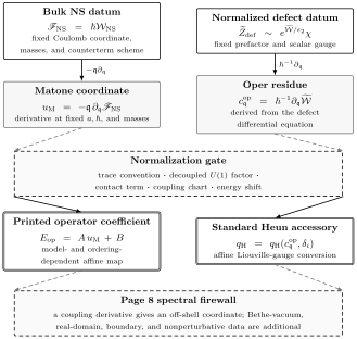
The derivative lanes are related but not interchangeable. The bulk free energy generates a chiral or Hamiltonian coordinate, while the normalized defect equation generates an oper residue. Trace conventions, decoupled $U(1)$ factors, coupling coordinates, contact terms, and energy shifts mediate their comparison. Neither lane supplies the Page 8 on-shell or boundary data.

A defect equation derives the accessory gradient

An accessory formula should be read from the differential equation that creates the oper, not imported from a classical-block convention. The mechanism is transparent in the regular four-puncture $U(2)$ example of Jeong and Nekrasov.

Let $\widetilde Z_\beta(a,z,\mathfrak q;\epsilon_1,\epsilon_2)$ be their surface-defect partition function after multiplication by specified powers of $z$, $\mathfrak q$, $1-z$, $1-\mathfrak q/z$, and $1-\mathfrak q$. Its finite-Omega Dyson–Schwinger equation contains

$$\begin{aligned} 0 = \Bigg[ &\epsilon_1^2\partial_z^2 - \epsilon_1\epsilon_2 \frac{2z-1}{z(z-1)} \partial_z \\ &+ \epsilon_1\epsilon_2 \frac{ \mathfrak q(\mathfrak q-1) }{ z(z-1)(z-\mathfrak q) } \partial_{\mathfrak q} \\ &+ \epsilon_1\epsilon_2 \,T_{\mathrm{finite}} \Bigg] \widetilde Z_\beta, \end{aligned}$$

where $T_{\mathrm{finite}}$ contains the prescribed double-pole and three-pole-free terms. The exact prefactor is part of this equation: a different normalization would conjugate the differential operator and add coupling derivatives of the prefactor.

In the NS limit, set $\epsilon_1=\hbar$ and factor the bulk singularity:

$$\widetilde Z_\beta = \exp\!\left[ \frac{ \widetilde{\mathcal W}(a,\mathfrak q) }{ \epsilon_2 } \right] \left[ \chi_\beta(a,z,\mathfrak q) +O(\epsilon_2) \right].$$

The defect observable contributes the finite wavefunction $\chi_\beta$; the $z$-independent bulk-plus-prefactor terms supply the $1/\epsilon_2$ exponent. Therefore

$$\epsilon_2 \partial_{\mathfrak q} \widetilde Z_\beta = \left[ \partial_{\mathfrak q} \widetilde{\mathcal W} +O(\epsilon_2) \right] \widetilde Z_\beta.$$

Divide the finite equation by $\hbar^2\widetilde Z_\beta$ and take the limit. The result is the Heun oper

$$\left[ \partial_z^2 + T_{\mathrm{op}}(z;\mathfrak q) \right] \chi_\beta =0,$$

with

$$\begin{aligned} T_{\mathrm{op}}(z;\mathfrak q) ={}& \frac{\delta_0}{z^2} + \frac{\delta_{\mathfrak q}} {(z-\mathfrak q)^2} + \frac{\delta_1}{(z-1)^2} \\ &+ \frac{ \delta_\infty-\delta_0-\delta_{\mathfrak q}-\delta_1 }{ z(z-1) } \\ &+ \frac{H} {z(z-1)(z-\mathfrak q)}. \end{aligned}$$

The coefficient inherited from the coupling derivative is

$$H = -\mathfrak q(1-\mathfrak q) \frac{1}{\hbar} \partial_{\mathfrak q} \widetilde{\mathcal W}$$

because $\mathfrak q(\mathfrak q-1)=-\mathfrak q(1-\mathfrak q)$. This sign is fixed by the finite differential equation.

One Heun accessory has three printed forms

The coefficient $H$ is compact, but it is not the residue at the moving pole. Comparing with the book’s four-pole oper convention,

$$\begin{aligned} T_{\mathrm{op}} ={}& \frac{\delta_0}{z^2} + \frac{\delta_{\mathfrak q}} {(z-\mathfrak q)^2} + \frac{\delta_1}{(z-1)^2} \\ &+ \frac{\Lambda_\delta}{z(z-1)} + \frac{ \mathfrak q(\mathfrak q-1) c_{\mathfrak q}^{\mathrm{op}} }{ z(z-1)(z-\mathfrak q) }, \end{aligned}$$

where

$$\Lambda_\delta := \delta_\infty-\delta_0-\delta_{\mathfrak q}-\delta_1,$$

gives

$$H = \mathfrak q(\mathfrak q-1) c_{\mathfrak q}^{\mathrm{op}}.$$

Combining this identity with the defect result yields the remarkably simple residue formula

$$\boxed{ c_{\mathfrak q}^{\mathrm{op}} = \frac1\hbar \partial_{\mathfrak q} \widetilde{\mathcal W} }$$

in this prefactor and scalar gauge. Thus $\widetilde{\mathcal W}/\hbar$ is a dimensionless branchwise generating function for the oper residue.

Scalar gauge produces the standard Heun parameter

The standard general-Heun equation is

$$\begin{aligned} y'' &+ \left( \frac{\gamma_{\mathrm H}}{z} + \frac{\delta_{\mathrm H}}{z-1} + \frac{\epsilon_{\mathrm H}}{z-\mathfrak q} \right)y' \\ &+ \frac{ \alpha_{\mathrm H}\beta_{\mathrm H}z-q_{\mathrm H} }{ z(z-1)(z-\mathfrak q) }y =0. \end{aligned}$$

The regular singularity at infinity imposes the Fuchs constraint

$$\gamma_{\mathrm H}+\delta_{\mathrm H}+\epsilon_{\mathrm H} = \alpha_{\mathrm H}+\beta_{\mathrm H}+1.$$

The classical-block oper page derived the Liouville-gauge conversion. Define

$$\kappa_{\mathrm H} := q_{\mathrm H} - \frac{\gamma_{\mathrm H}}{2} \left( \mathfrak q\delta_{\mathrm H}+\epsilon_{\mathrm H} \right).$$

Then

$$c_{\mathfrak q}^{\mathrm{op}} = \frac{ \mathfrak q\Lambda_\delta-\kappa_{\mathrm H} }{ \mathfrak q(\mathfrak q-1) }.$$

Solving for the standard accessory gives

$$\boxed{ \begin{aligned} q_{\mathrm H} ={}& \frac{\gamma_{\mathrm H}}{2} \left( \mathfrak q\delta_{\mathrm H}+\epsilon_{\mathrm H} \right) + \mathfrak q\Lambda_\delta \\ &- \frac{ \mathfrak q(\mathfrak q-1) }{ \hbar } \partial_{\mathfrak q} \widetilde{\mathcal W}. \end{aligned} }$$

Equivalently, since $H=\mathfrak q(\mathfrak q-1)c_{\mathfrak q}^{\mathrm{op}}$,

$$q_{\mathrm H} = \frac{\gamma_{\mathrm H}}{2} \left( \mathfrak q\delta_{\mathrm H}+\epsilon_{\mathrm H} \right) + \mathfrak q\Lambda_\delta -H.$$

The first two terms are not optional decorations: they are the affine shift created by removing the first derivative. Calling $H$, $c_{\mathfrak q}^{\mathrm{op}}$, and $q_{\mathrm H}$ all “the accessory parameter” hides both a factor $\mathfrak q(\mathfrak q-1)$ and this shift.

The chiral observable reaches the oper through contacts

The same Dyson–Schwinger derivation makes the relation to the quadratic chiral observable explicit. To quote it without silently projecting from $U(2)$ to $SU(2)$, retain the source’s center variables

$$\bar a_i := \frac{a_{i,1}+a_{i,2}}{2}, \qquad \bar a := \frac{a_1+a_2}{2}.$$

Let $\mathcal O_2=\operatorname{Tr}\phi_2^2$ be the source-normalized quadratic observable of the internal gauge node. In the NS limit,

$$\begin{aligned} H ={}& (1-\mathfrak q) \left[ \frac{1}{2\hbar^2} \lim_{\epsilon_2\to0} \langle\mathcal O_2\rangle -\frac14 +\delta_{\mathfrak q} +\delta_0 \right] \\ &+ \frac{ 2(\bar a_0-\bar a) (\bar a-\bar a_3+\hbar) }{ \hbar^2 } \mathfrak q. \end{aligned}$$

This formula is more informative than an unqualified statement that “the accessory equals the energy.” It displays:

1. the factor $1/(2\hbar^2)$ converting the source’s full trace into a dimensionless oper coefficient;
2. the puncture-weight contact $-1/4+\delta_{\mathfrak q}+\delta_0$;
3. a $U(1)$-center contribution involving $(\bar a_0,\bar a,\bar a_3)$; and
4. the geometric factor $1-\mathfrak q$.

On a traceless slice some center terms simplify, but they should be set to zero only after the $U(2)$ prefactor and mass map have been translated. Removing a decoupled Abelian factor changes $\widetilde{\mathcal W}$ by a coupling-dependent function and produces exactly this sort of affine shift.

The normalization ladder is therefore

$$\begin{gathered} \lim_{\epsilon_2\to0} \langle\mathcal O_2\rangle \quad\xrightarrow[ \text{trace and contacts} ]{ \text{affine map} } H, \\ H = \mathfrak q(\mathfrak q-1) c_{\mathfrak q}^{\mathrm{op}} \quad\xrightarrow[ \text{Liouville gauge} ]{ \text{affine map} } q_{\mathrm H}. \end{gathered}$$

Every arrow is invertible away from its stated degeneration once the external data are fixed. None is an identity of notation.

A rational four-puncture checksum

The classical-block laboratory supplies a useful exact arithmetic check of every conversion. Choose exponent differences

$$\theta_0=\theta_{\mathfrak q}=\frac13, \qquad \theta_1=\theta_\infty=\frac15, \qquad \theta_{0\mathfrak q}=\frac35.$$

On its selected zero–$\mathfrak q$ channel, the moving-pole residue is

$$c_{\mathfrak q}^{\mathrm{op}} = -\frac{64}{225\mathfrak q} +\frac2{25} +\frac{587}{5850}\mathfrak q +O(\mathfrak q^2).$$

Multiplying by $\mathfrak q(\mathfrak q-1)$ gives

$$H = \frac{64}{225} -\frac{82}{225}\mathfrak q -\frac{119}{5850}\mathfrak q^2 +O(\mathfrak q^3).$$

The standard-Heun number also requires exponent representatives. Choose the positive lifts inherited from the classical-block laboratory,

$$\begin{gathered} \gamma_{\mathrm H}=\epsilon_{\mathrm H}=\alpha_{\mathrm H}=\frac23, \qquad \delta_{\mathrm H}=\frac45, \qquad \beta_{\mathrm H}=\frac7{15}, \\ \Lambda_\delta=-\frac49. \end{gathered}$$

The scalar-gauge conversion then yields

$$q_{\mathrm H} = -\frac{14}{225} +\frac{14}{75}\mathfrak q +\frac{119}{5850}\mathfrak q^2 +O(\mathfrak q^3).$$

The three series check the pole normalization, the compact factor, and the affine Heun shift independently. They are an oper/CFT arithmetic benchmark. Applying the preceding gauge-chiral formula requires a separate mass and $U(1)$-center assignment because the puncture weights are functions of those parameters; they cannot be combined with an arbitrary centered slice.

Why the omitted one-loop term is harmless here—and only here

Near the displayed Heun equation, the source defines

$$\widetilde{\mathcal W} = \widetilde{\mathcal W}^{\mathrm{cl}} + \widetilde{\mathcal W}^{\mathrm{inst}} + \widetilde{\mathcal W}^{\mathrm{extra}},$$

temporarily omitting the bulk one-loop term. That term is independent of $\mathfrak q$ in the chosen weak-coupling chart, so $\partial_{\mathfrak q}$ cannot see it and the accessory formula is unchanged. It must be restored when the full generating function or an $a$ derivative is needed. A boundary contribution independent of $\mathfrak q$ is similarly invisible to this accessory but can shift the conjugate monodromy coordinate.

The criterion is derivative-specific:

$$\partial_{\mathfrak q}C=0 \quad\Longrightarrow\quad C\text{ is invisible to this accessory derivative}.$$

It does not imply that $C$ is physically irrelevant or may be dropped from every equation.

Full and unit-leading generating functions differ at the pole

The classical-block page distinguished a full channel block from its unit-leading power series. The same issue appears on the gauge side because defect prefactors contain powers of $\mathfrak q$ and $1-\mathfrak q$.

Suppose

$$\frac{ \widetilde{\mathcal W} }{ \hbar } = \kappa_{\mathrm{OPE}} \Log\mathfrak q + \widehat f(\mathfrak q).$$

Then the oper residue is

$$c_{\mathfrak q}^{\mathrm{op}} = \frac{\kappa_{\mathrm{OPE}}}{\mathfrak q} + \partial_{\mathfrak q} \widehat f.$$

Dropping the leading power while keeping the full-block derivative loses the pole $\kappa_{\mathrm{OPE}}/\mathfrak q$. Conversely, adding a prefactor $(1-\mathfrak q)^\rho$ changes the residue by $-\rho/(1-\mathfrak q)$. These are not discrepancies between gauge theory and CFT; they are calculable normalization changes.

For the complete branchwise classical-block derivation and its monodromy interpretation, see Classical Blocks, Opers, and Accessory Parameters. The present page establishes the gauge/defect route without assuming the Chapter 11 AGT dictionary.

Multipuncture gradients must be integrable

For an $n$-punctured sphere, choose local moduli $\boldsymbol t=(t_1,\ldots,t_{n-3})$. A normalized defect equation can produce a collection

$$c_r^{\mathrm{op}} = \partial_{t_r} \left( \frac{\widetilde{\mathcal W}} {\hbar} \right) +c_r^{\mathrm{contact}}, \qquad r=1,\ldots,n-3.$$

If all contacts themselves derive from one local function $C(\boldsymbol t)$, then

$$\partial_{t_s}c_r^{\mathrm{op}} = \partial_{t_r}c_s^{\mathrm{op}}.$$

Failure of this mixed-derivative test signals at least one of the following:

• different puncture charts were mixed without their Jacobian;
• one defect prefactor or decoupled factor was omitted;
• the scalar-gauge conversion was applied to only some residues;
• derivatives were taken while holding different mass coordinates fixed; or
• the proposed accessories do not arise from one branchwise generating function.

The converse is local: a closed accessory one-form is locally exact on a simply connected patch, but global continuation can add periods and move between logarithm or monodromy branches.

Matone, mirror, and accessory relations compared

The three relations can now be stated without overloading $u$:

Relation	Defining or derived equation	What fixes its normalization?	What it does not supply
Quantum mirror map	$a=a_A^{\mathrm{WKB}}(u,\hbar)$, inverted for $u$	WKB form, A-cycle, $2\pi\ii$, operator modulus	Coupling insertion or accessory scalar gauge
Matone type	$u_{\mathrm M}=-\mathfrak q\partial_{\mathfrak q}\mathscr F_{\mathrm{NS}}$	Trace, coupling, scale, counterterm, and Abelian scheme	A-period invertibility or an ODE
Accessory gradient	$c_t^{\mathrm{op}}=\partial_t(\widetilde{\mathcal W}/\hbar)$	Defect equation, prefactor, puncture chart, scalar gauge	Standard Heun $q_{\mathrm H}$ without affine conversion
Chiral-to-oper map	$H=A\langle\mathcal O_2\rangle+B$	Operator normalization and contact terms	On-shell quantization
Energy map	$E_{\mathrm{op}}=A_Eu_{\mathrm M}+B_E$	Polarization, ordering, and coordinate convention	Domain and boundary conditions

In the pure modified-Mathieu benchmark, the first, second, and fifth rows coincide after calibration. In the regular four-puncture example, the second, third, and fourth rows are linked by the defect Dyson–Schwinger equation and the displayed contacts. These successes are powerful consistency checks precisely because the constructions are independent before calibration.

Off shell is not incomplete mathematics

In the stated four-puncture defect model, at generic Coulomb parameter $a$, the coupling derivative determines a holomorphic coordinate on the variety of opers. In the integrable-system language it is an off-shell Hamiltonian value: a function on the oper Lagrangian before intersecting it with a second Lagrangian that implements a vacuum or boundary condition.

The distinction is structural:

$$\begin{array}{c} \text{NS or defect generating function at generic }a \\ \Downarrow\ \partial_{\mathfrak q} \\ \text{off-shell oper or Hamiltonian coordinate} \\ \Downarrow\ \text{Bethe-vacuum condition} \\ \text{discrete candidate values} \\ \Downarrow\ \text{domain, boundary, and completion} \\ \text{a specified exact ODE spectrum}. \end{array}$$

This page stops after the first arrow. Page 8 will analyze the remaining arrows, including why an NS-limit expression need not be a complete nonperturbative spectral answer.

Analytic domains remain attached to defect solutions

The weak-coupling defect series used above gives solutions in the chart

$$0<|\mathfrak q|<1<|z|.$$

Other Frobenius or connection domains require analytic continuation and different defect bases. The oper coefficient $H$ is holomorphic data continued with the equation, but a particular series for $\chi_\beta$ is not valid globally. Accessory agreement does not by itself provide normalized connection matrices; finite Gamma factors arise when defect bases are glued.

A normalization-complete workflow

For a new quantum-curve problem, the following order prevents most false identifications.

1. Name the coupling coordinate. State whether it is a dimensionless cross-ratio, a dimensionful fugacity $\Lambda^{b_0}$, or a finite reparametrization.
2. Fix what the derivative holds constant. Bare and centered masses can differ by $\hbar/2$; differentiating along those two slices gives different contacts.
3. Normalize the chiral observable. Declare the trace, the classical value, and the equivariant completion at each fixed point.
4. Differentiate the connected quantity. Use $\log Z$, then take the NS limit; do not differentiate a disconnected partition sum and call it a free-energy insertion.
5. Audit local terms. Separate coupling-independent Barnes polynomials from coupling-dependent contact and Abelian factors.
6. Derive the defect equation at finite Omega deformation. Record its prefactor and the exact coefficient multiplying each coupling derivative.
7. Take the NS asymptotics inside that equation. This fixes the sign and geometric factors of the oper accessory.
8. Choose the accessory basis. Convert among partial-fraction residues, compact coefficients, and standard Heun parameters.
9. Calibrate the energy map. Compare classical limits, dimensions, weak-coupling coefficients, resonance divisors, and any finite $\hbar$ shift.
10. Keep the spectral firewall closed. Add vacuum, reality, boundary, Stokes, and nonperturbative data only when they have been independently specified.

Interpretation and limitations

The pure-$SU(2)$ Matone relation is unusually clean because the same instanton counting parameter controls both the gauge expansion and the modified-Mathieu potential, the Page 5 ordering is unshifted, and the Page 2 trace and period normalization have already been calibrated. Matter theories and conformal quivers add mass contacts, Abelian factors, and nontrivial coupling charts.

The four-puncture accessory derivation is stronger than a low-order matching: within the theory and normalization for which the nonperturbative Dyson–Schwinger equation is established, inserting the NS asymptotics proves the coupling-derivative coefficient to all orders in the weak-coupling expansion. It is still not a theorem about every surface defect, every oper chart, or arbitrary analytic continuation.

Neither derivation settles Borel summation in $\hbar$. A formal or meromorphic weak-$\mathfrak q$ expression can agree coefficientwise with quantum periods while different lateral WKB sums differ across a Stokes wall. Nor does either derivation select a self-adjoint operator or an $L^2$ domain.

Common pitfalls

Differentiating at fixed $u$ instead of fixed $a$. The NS free energy is naturally expressed in the flat electric coordinate, so the Matone derivative on this page holds $a$ fixed. After the quantum mirror map, fixed-$a$ and fixed-$u$ derivatives differ by a chain-rule term.

Using the instanton-only formula as the full relation. The instanton derivative computes $u-a^2$ in the pure benchmark. The classical $a^2$ term comes from the calibrated perturbative scale dependence.

Treating a q-independent term as universally irrelevant. Such a term is invisible to $\partial_{\mathfrak q}$ but can change $\partial_a\mathscr F_{\mathrm{NS}}$, monodromy coordinates, and vacuum equations. Relevance depends on the derivative being computed.

Calling H the standard Heun q. The compact normal-form coefficient satisfies $H=\mathfrak q(\mathfrak q-1)c_{\mathfrak q}^{\mathrm{op}}$. The standard $q_{\mathrm H}$ also contains the explicit Liouville-gauge shift.

Setting U(1) centers to zero too early. A $U(2)$ defect normalization can contain center-dependent powers even when the desired bulk theory is ultimately traceless. Translate or divide the Abelian factor before imposing the $SU(2)$ slice.

Reading a spectrum from an accessory value. At generic $a$, the accessory is an off-shell coordinate. Discreteness appears only after a vacuum or boundary condition is imposed, and an exact ODE spectrum may require further nonperturbative completion.

Exercises

1. Insert instanton number

Let

$$Z(q)=\sum_{k\geq0}q^kZ_k, \qquad Z_0=1.$$

Show that $q\partial_q\log Z$ is the normalized expectation of $k$. Expand the answer through $q^2$.

Solution

Define $\langle k\rangle=Z^{-1}\sum_{k\geq0}kq^kZ_k$. Direct differentiation gives

$$q\partial_q\log Z = \frac{q\partial_q Z}{Z} = \langle k\rangle.$$

Since

$$\log Z = qZ_1 +q^2 \left( Z_2-\frac12Z_1^2 \right) +O(q^3),$$

one obtains

$$q\partial_q\log Z = qZ_1 +2q^2 \left( Z_2-\frac12Z_1^2 \right) +O(q^3).$$

The connected subtraction and the factor two are both essential.

2. Reproduce the finite-ħ mirror map

Starting from

$$\begin{aligned} \mathcal W_{\mathrm{NS}}^{\mathrm{inst}} ={}&- \frac{2\mathfrak q} {\hbar(4a^2-\hbar^2)} \\ &- \frac{ \mathfrak q^2(20a^2+7\hbar^2) }{ 4\hbar(a^2-\hbar^2) (4a^2-\hbar^2)^3 } +O(\mathfrak q^3), \end{aligned}$$

compute $a^2-\hbar\mathfrak q\partial_{\mathfrak q} \mathcal W_{\mathrm{NS}}^{\mathrm{inst}}$.

Solution

The logarithmic derivative multiplies the one- and two-instanton terms by one and two. Hence

$$\begin{aligned} u ={}&a^2 +\frac{2\mathfrak q}{4a^2-\hbar^2} \\ &+ \frac{ \mathfrak q^2(20a^2+7\hbar^2) }{ 2(a^2-\hbar^2) (4a^2-\hbar^2)^3 } +O(\mathfrak q^3). \end{aligned}$$

This is the Page 6 fixed-$\hbar$ Floquet characteristic germ.

3. Expand the quantum correction

Expand the answer of Exercise 2 through $O(\hbar^2\mathfrak q^2)$.

Solution

Use geometric-series expansions of each denominator. At one instanton,

$$\frac{2\mathfrak q}{4a^2-\hbar^2} = \frac{\mathfrak q}{2a^2} + \frac{\hbar^2\mathfrak q}{8a^4} +O(\hbar^4).$$

At two instantons,

$$\frac{ \mathfrak q^2(20a^2+7\hbar^2) }{ 2(a^2-\hbar^2)(4a^2-\hbar^2)^3 } = \frac{5\mathfrak q^2}{32a^6} + \frac{21\hbar^2\mathfrak q^2}{64a^8} +O(\hbar^4).$$

Adding $a^2$ gives the formal WKB mirror map quoted on the page.

4. Derive the scaling form

Assume the pure NS free energy is homogeneous of degree two in $(a,\hbar,\Lambda)$ and $u=-(\Lambda/4)\partial_\Lambda\mathscr F_{\mathrm{NS}}$. Derive the Euler form of the Matone relation.

Solution

Euler’s identity gives

$$a\partial_a\mathscr F_{\mathrm{NS}} + \hbar\partial_\hbar\mathscr F_{\mathrm{NS}} + \Lambda\partial_\Lambda\mathscr F_{\mathrm{NS}} = 2\mathscr F_{\mathrm{NS}}.$$

Therefore

$$\begin{aligned} u &=-\frac14 \Lambda\partial_\Lambda \mathscr F_{\mathrm{NS}} \\ &= \frac14 \left( a\partial_a +\hbar\partial_\hbar -2 \right) \mathscr F_{\mathrm{NS}}. \end{aligned}$$

The coefficient is tied to $\mathfrak q=\Lambda^4$.

5. Track a contact term

Let

$$C(\mathfrak q,\hbar) = \rho\hbar^2\Log(1-\mathfrak q).$$

If $\mathscr F_{\mathrm{NS}}'=\mathscr F_{\mathrm{NS}}+C$, find the change in $u_{\mathrm M}$.

Solution

By definition,

$$\Delta u_{\mathrm M} = -\mathfrak q\partial_{\mathfrak q}C = \rho\hbar^2 \frac{\mathfrak q}{1-\mathfrak q}.$$

This is a coupling-dependent finite-$\hbar$ shift. It cannot be removed by saying that the free energy is defined only up to a constant.

6. Change the coupling chart

Take

$$\widetilde q = q+cq^2+O(q^3).$$

Find the logarithmic Jacobian relating $q\partial_q$ to $\widetilde q\partial_{\widetilde q}$ through first order in $q$.

Solution

Since $f'(q)=1+2cq+O(q^2)$,

$$\frac{qf'(q)}{f(q)} = \frac{1+2cq+O(q^2)} {1+cq+O(q^2)} = 1+cq+O(q^2).$$

Hence

$$q\partial_q = \left[ 1+cq+O(q^2) \right] \widetilde q\partial_{\widetilde q}.$$

The first instanton normalization is unchanged, while higher coefficients mix.

7. Extract H from the defect equation

Suppose a finite-Omega equation contains

$$\epsilon_1^2\partial_z^2 + \epsilon_1\epsilon_2 \frac{q(q-1)}{z(z-1)(z-q)} \partial_q.$$

Insert $\widetilde Z=e^{\widetilde{\mathcal W}/\epsilon_2} (\chi+O(\epsilon_2))$ and identify the compact oper coefficient.

Solution

At leading order,

$$\epsilon_2\partial_q\widetilde Z = \left( \partial_q\widetilde{\mathcal W} +O(\epsilon_2) \right) \widetilde Z.$$

After division by $\epsilon_1^2\widetilde Z$ and setting $\epsilon_1=\hbar$, the three-denominator coefficient is

$$H = \frac{q(q-1)}{\hbar} \partial_q\widetilde{\mathcal W} = -\frac{q(1-q)}{\hbar} \partial_q\widetilde{\mathcal W}.$$

The sign follows from the polynomial $q(q-1)$ in the finite equation.

8. Convert H into two accessory conventions

Given

$$H=q(q-1)c_q^{\mathrm{op}}$$

and

$$c_q^{\mathrm{op}} = \frac{ q\Lambda_\delta-\kappa_{\mathrm H} }{q(q-1)}, \qquad \kappa_{\mathrm H} = q_{\mathrm H}-\frac{\gamma_{\mathrm H}}{2} (q\delta_{\mathrm H}+\epsilon_{\mathrm H}),$$

solve first for $c_q^{\mathrm{op}}$ in terms of $\widetilde{\mathcal W}$ and then for $q_{\mathrm H}$ in terms of $H$.

Solution

Exercise 7 gives

$$c_q^{\mathrm{op}} = \frac{H}{q(q-1)} = \frac1\hbar\partial_q \widetilde{\mathcal W}.$$

The second relation implies $\kappa_{\mathrm H}=q\Lambda_\delta-H$. Therefore

$$q_{\mathrm H} = \frac{\gamma_{\mathrm H}}{2} (q\delta_{\mathrm H}+\epsilon_{\mathrm H}) +q\Lambda_\delta-H.$$

9. Restore an OPE prefactor

Suppose a unit-leading generating function $\widehat f(q)$ is related to the full one by

$$f(q)=\kappa\Log q+\widehat f(q).$$

How do their accessory residues differ?

Solution

Differentiation gives

$$\partial_q f = \frac{\kappa}{q} +\partial_q\widehat f.$$

Thus the full normalization has an additional pole $\kappa/q$. The pole records the leading channel power and must be restored before comparing with a full-block or full-defect oper.

10. Test a two-modulus accessory proposal

Suppose proposed residues on a simply connected patch are

$$c_1(t_1,t_2)=t_2+\frac{\rho}{t_1}, \qquad c_2(t_1,t_2)=t_1+g(t_2).$$

Do they admit a local generating function? If so, construct one.

Solution

The integrability test is

$$\partial_{t_2}c_1=1 = \partial_{t_1}c_2.$$

It passes. Integrating the first residue gives

$$f(t_1,t_2) = t_1t_2 +\rho\Log t_1 +G(t_2),$$

and matching $c_2$ requires $G'(t_2)=g(t_2)$. Hence

$$f = t_1t_2 +\rho\Log t_1 +\int^{t_2}g(s)\,\dd s$$

up to a constant and branch choice. Passing this local test does not guarantee a single-valued global generating function.

References

• M. Matone, “Instantons and Recursion Relations in N=2 SUSY Gauge Theory”, Physics Letters B 357 (1995), 342–348. Introduces the original pure-$SU(2)$ relation between the quantum modulus and instanton prepotential coefficients. Its trace, scale, and prepotential normalizations differ from the house convention and must be translated together.
• R. Flume, F. Fucito, J. F. Morales, and R. Poghossian, “Matone’s Relation in the Presence of Gravitational Couplings”, Journal of High Energy Physics 04 (2004) 008. Section 4.2, especially equations (4.12)–(4.14), evaluates the equivariantly completed quadratic chiral observable at fixed points and proves the instanton relation at arbitrary winding and Omega deformation. Equation (4.18), rather than the undeformed chiral-ring equation (4.17), is the finite-deformation coefficient check relevant here.
• N. Nekrasov and A. Okounkov, “Seiberg–Witten Theory and Random Partitions”, in The Unity of Mathematics, Progress in Mathematics 244 (2006), 525–596. Sections 2–4 formulate the partition measure and its chiral observables; logarithmic coupling derivatives insert partition size.
• W. He, “Matone’s Relation of N=2 Super Yang–Mills and Spectrum of Toda Chain”, Communications in Theoretical Physics 56 (2011), 905–912. Sections 2–3 check the Omega-deformed instanton relation and its localization origin; Section 4 relates the quadratic chiral observable to periodic-Toda energy. Equation (13) exhibits the perturbative $\hbar^2/24$ anomaly, while equations (14)–(20) are instanton-sector statements; the two should not be silently folded together.
• A. Grassi, J. Gu, and M. Mariño, “Non-Perturbative Approaches to the Quantum Seiberg–Witten Curve”, Journal of High Energy Physics 07 (2020) 106. Equations (4.12)–(4.14) give an exact-in-$\hbar$ pure-$SU(2)$ instanton free energy and quantum Matone relation. Their variables obey a nontrivial package map to the book’s $a$, $u$, and holomorphic $\hbar$; after translation they reproduce the finite-$\hbar$ two-instanton germ checked above.
• S. Jeong and N. Nekrasov, “Opers, Surface Defects, and Yang–Yang Functional”, Advances in Theoretical and Mathematical Physics 24 (2020), 1789–1916. Equation (3.17) is the finite-Omega defect Dyson–Schwinger equation; equations (3.19)–(3.20) give its NS factorization and the classical, instanton, and prefactor pieces. Equations (3.22)–(3.23) give the four-puncture Heun oper, its coupling derivative, and its affine relation to $\operatorname{Tr}\phi^2$. The remarks after (3.23) state the all-orders weak-coupling status and the domain $0<|\mathfrak q|<1<|z|$. Section 6 restores the coupling-independent one-loop contribution for the full generating function; equations (6.24)–(6.25) prove the $SL(2)$ NRS generating-function relation in the stated four-puncture class.
• N. Nekrasov, A. Rosly, and S. Shatashvili, “Darboux Coordinates, Yang–Yang Functional, and Gauge Theory”, Nuclear Physics B Proceedings Supplements 216 (2011), 69–93. Develops the generating-function interpretation in a chosen Darboux chart and explains the additional Lagrangian data entering Bethe equations. The broad NRS identification is conjectural there; the preceding Jeong–Nekrasov reference proves the stated $SL(2)$ four-puncture class.
• A. Litvinov, S. Lukyanov, N. Nekrasov, and A. Zamolodchikov, “Classical Conformal Blocks and Painlevé VI”, Journal of High Energy Physics 07 (2014) 144. Equations (2.1) and (2.9) state the partial-fraction oper and accessory gradient; equations (2.13)–(2.14) specialize it to four punctures and verify the factor $\mathfrak q(\mathfrak q-1)$ between the compact coefficient and moving-pole residue.
• F. Ferrari and M. Piątek, “Liouville Theory, N=2 Gauge Theories and Accessory Parameters”, Journal of High Energy Physics 05 (2012) 025. Relates the four-point classical-block derivative, the NS instanton saddle, and the four-puncture accessory parameter. Its $U(2)$ factors and classical-block normalization must be retained when comparing with a standard Heun $q_{\mathrm H}$.
• K. Maruyoshi and M. Taki, “Deformed Prepotential, Quantum Integrable System and Liouville Field Theory”, Nuclear Physics B 841 (2010), 388–425. Equations (3.47)–(3.49) exhibit an intermediate $-\hbar^2/4$ term and the final unshifted sine–Gordon/Mathieu energy; the half-form calculation above explains the cancellation. The paper provides a useful low-order corroboration, not the all-orders defect proof used above.
• NIST Digital Library of Mathematical Functions, §31.2, Heun equations, for the standard first-derivative Heun convention used in the final affine conversion.