Epilogue: Beyond the Book

This book has concentrated on second-order scalar equations, rank-two connections, and one-dimensional spectral problems, usually on the Riemann sphere. That is a deliberate stopping point, not the boundary of the subject. One can add marked poles, increase the rank or differential order, replace derivatives by finite shifts, or change the topology of the underlying curve. Each move preserves the central question—how do normalized local solutions fit together globally?—while changing the kind of object that can answer it.

The formulas do not survive unchanged. A constant $2\times2$ connection matrix may become a collection of generalized minors, a periodic matrix-valued function, or a representation of the fundamental group of a higher-genus curve. The reusable part is instead the equation-and-basis passport, an extension of the book’s normalization ledger: state the operator, normalized frames, global datum, analytic domain, and an independent check. This epilogue surveys five frontier topics along four structural extensions and turns them into eight concrete connection problems.

How to read this epilogue

The first paragraph of each frontier gives the structural change. The following paragraphs identify what is already a theorem, what needs extra hypotheses, and what remains a useful research target. A reader planning a project can then jump to the open-problem ledger and the research workflow.

The passport survives when the analytic category changes

Extension	Replacement for the rank-two picture	Global datum to request	First category error to avoid
More marked poles	Several accessory parameters and several deformation times	Framed connection matrices as functions of Garnier times	Calling every static many-pole equation a Garnier system
Higher rank or order	Flags, exterior products, and generalized minors	A normalized family of connection minors or $Q$-functions	Treating one scalar determinant as the whole $Q$-system
Finite shifts	Additive- or $q$-periodic fields of constants	Birkhoff connection functions and discrete Stokes data	Assuming that a connection matrix is constant
Elliptic or higher-genus geometry	Handle cycles, bundles, and spectral covers	Holonomy plus local and Stokes data in a declared marking	Confusing the genus of the base with the genus of a WKB cover

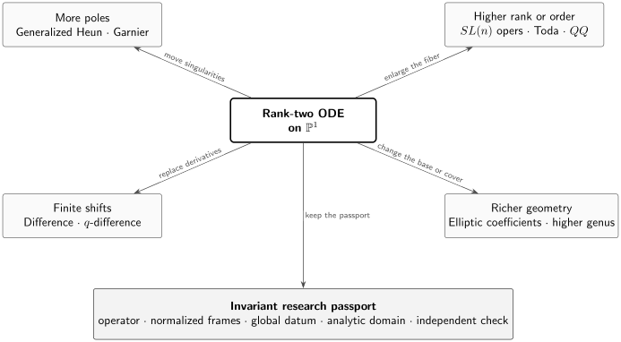
The four branches are independent and can be combined. A higher-rank $q$-difference oper on a curve equipped with the required automorphism—for example, an elliptic translation—occupies several branches at once. It therefore needs every corresponding addition to the passport, not a choice of only one.

The last column is the most important one. Each frontier has a tempting analogy with a familiar rank-two ODE, but the analogy becomes a theorem only after its new constants, gauges, topology, and exceptional loci have been specified.

More poles turn Heun into a multidimensional problem

The name “generalized Heun equation” is not standardized. Here a generalized Heun-type Fuchsian oper means a second-order scalar equation on $\mathbb P^1$ with exactly $m\geq5$ prescribed regular singular points, including infinity, and no additional coefficient singularities. In projective normal form it is locally

$$\begin{aligned} \psi''(z)+T(z)\psi(z)&=0,\\ T(z)&= \sum_{i=1}^{m-1} \left[ \frac{\delta_i}{(z-t_i)^2} +\frac{c_i}{z-t_i} \right]. \end{aligned}$$

Fixing the local exponents fixes the $\delta_i$ and the exponent invariant $\delta_\infty$ at infinity. Regularity there imposes

$$\sum_{i=1}^{m-1}c_i=0, \qquad \sum_{i=1}^{m-1} \left(\delta_i+t_i c_i\right)=\delta_\infty.$$

Consequently the scalar oper has $m-3$ accessory parameters. Möbius normalization also leaves $m-3$ positions of marked poles. Thus $m=3$ is the hypergeometric case, $m=4$ is Heun, and

$$\{0,1,t_1,t_2,\infty\}$$

is the first genuinely multivariable example: two pole positions and two accessory parameters.

The oper locus is only half of the monodromy space

Now begin with a generic rank-two Fuchsian system,

$$\partial_z\Phi= \sum_{i=1}^{m-1} \frac{A_i}{z-t_i}\Phi, \qquad A_\infty=-\sum_{i=1}^{m-1}A_i.$$

After a generic semisimple $A_\infty$ is put in diagonal form, the standard cyclic component adapted to infinity converts the system to a scalar equation with $r=m-3$ finite apparent singularities $\lambda_a$. They are poles of the scalar coefficients whose local monodromy is trivial; in a common scalar gauge their exponents are $(0,2)$. Their conjugate variables $\mu_a$ form a $2r$-dimensional phase space. The Schlesinger deformations in the $r$ marked positions become the Garnier system $\mathcal G_r$, with $\mathcal G_1$ equal to Painlevé VI.

The qualification on the cyclic component matters. Another cyclic vector can move the apparent poles or add an extra finite zero; the $2r$-dimensional character variety and its Garnier flow are the invariant objects.

This dimension count prevents three common conflations:

• the $m-3$ accessory parameters of a pole-only scalar oper are not the $2(m-3)$ Darboux coordinates of a generic local system;
• an isolated many-pole scalar equation is not an isomonodromic family;
• an apparent pole has trivial monodromy but is not absent from the scalar equation.

The many-pole theory is already exact in important senses. For generic Fuchsian systems on the sphere, Fredholm determinants give isomonodromic tau functions, and in rank two their expansions use hypergeometric three-point building blocks. Suitable linear combinations of $c=1$ conformal blocks also solve the genus-zero multipuncture $\mathrm{SL}(2,\mathbb C)$ Riemann–Hilbert problem. These are powerful global results, but

$$\mathrm d\log\tau_{\mathrm{iso}} =\sum_{a=1}^{r}H_a\,\mathrm d t_a$$

does not by itself select a scalar cyclic vector or normalize two scalar Frobenius bases. A tau function, a scalar connection entry, and a boundary spectral determinant remain different sections until a theorem fixes the missing gauges and holomorphic factors.

A five-pole benchmark

A useful next laboratory would freeze exponents and branch conventions for $\{0,1,t_1,t_2,\infty\}$, choose normalized Frobenius frames at $0$ and $1$, and compute one connection entry in two independent ways:

1. direct high-precision continuation of the scalar ODE; and
2. a two-time Garnier or Fredholm-tau representation with its scalar gauge derived explicitly.

The benchmark should include a braid in $(t_1,t_2)$, a resonance limit, and a collision such as $t_2\to t_1$. Agreement only at one generic point would test a number; these deformations test the proposed dictionary. The first open problem turns this benchmark into a bounded deliverable.

Higher rank separates the oper from its dictionaries

An $\mathrm{SL}_N$-oper is intrinsically a flat rank-$N$ connection together with a full flag satisfying a transversality condition. In a local coordinate and oper gauge, a cyclic vector gives

$$\mathcal D = \partial_z^N +t_2(z)\partial_z^{N-2} +\cdots +t_{N-1}(z)\partial_z +t_N(z).$$

The missing $\partial_z^{N-1}$ term records the $\mathrm{SL}_N$ normalization. This expression is local: globally the scalar operator acts between line bundles, and $t_2$ transforms as a projective connection rather than an ordinary quadratic differential. For a general simple group $G$, its fundamental representations are more intrinsic than any claim of a single universal scalar equation of order $\operatorname{rank}G$.

Rank-two objects therefore generalize by representation theory:

Rank two	Higher rank
two exponent labels	weight-valued exponent data
Wronskian	exterior product or generalized minor
Wronskian identity	Plücker relation
quadratic WKB cover	$N$-sheeted spectral cover
one sheet pair at a Stokes ray	root-labelled wall between a sheet pair
one Baxter function in the simplest models	a family indexed by Dynkin nodes or fundamental representations

Different cyclic vectors can introduce different apparent poles. Likewise, changing a local flag normalization rescales minors. A higher-rank connection formula must consequently name the representation, ordered flags, minor, and normalization—not merely the scalar oper coefficients.

Toda CFT supplies a bridge only in specified sectors

Type-$A_{N-1}$ Toda theory has a $W_N$ chiral algebra, and the quantum Miura construction packages its currents of spins $2,\ldots,N$ into a product of first-order operators. This is the structural reason that Toda null-vector equations and $\mathrm{SL}_N$ opers meet.

The Virasoro lesson cannot simply be copied, however. A single completely degenerate Toda insertion does not generically close to a finite-order scalar ODE when the remaining insertions are arbitrary. Closure occurs in specified degenerate or semi-degenerate configurations. Even there, one must distinguish a chiral block, a full single-valued correlator, and a normalized fusion or connection matrix. The higher-rank AGT relation was introduced as a proposal and remains model- and normalization-dependent in the form needed for connection amplitudes.

The third-order $T_3$ equation is a useful calibration case: exact-WKB abelianization produces concrete higher-rank spectral coordinates and numerical checks. It is evidence for a rich dictionary, not a universal formula for arbitrary third-order equations.

Higher-order ODE/IM needs an entire Q-system

For suitable order-$N$ ODE families, canonically subdominant solutions in rotated Stokes sectors generate exterior-product identities. In type $A$, one schematic bosonic form is

$$\begin{aligned} Q_{Aab}(u)Q_A(u) &= Q_{Aa}^{+}(u)Q_{Ab}^{-}(u) - Q_{Aa}^{-}(u)Q_{Ab}^{+}(u),\\ Q^\pm(u)&=Q(u\pm\delta), \qquad a,b\notin A. \end{aligned}$$

Here $A$ is a subset of the index set, $a$ and $b$ are distinct indices outside $A$, $Aa$ abbreviates $A\cup\{a\}$, and $Aab=A\cup\{a,b\}$. The quantity $\delta$ is a model-dependent spectral shift. Signs, shifts, twists, and even the form of the relation change for supersymmetric, non-simply-laced, or affine systems. The displayed identity is therefore a map of the architecture, not a definition valid in every model.

To turn Plücker identities into a physical QQ-system one still needs:

1. a declared ODE or affine connection family;
2. normalized subdominant solutions in every required representation;
3. the rotation or shift symmetry acting on the spectral parameter;
4. a precise identification of exterior Wronskians with the $Q_i$;
5. large-parameter asymptotics and allowed zero sets;
6. a gauge fixing for all $Q$-functions; and
7. analyticity and genericity conditions before evaluating at zeros to obtain Bethe equations.

Dorey, Dunning, and Tateo established the $\mathrm{SU}(N)$ Bethe relations for a suitable family of $N$th-order equations. Later affine-oper work proves $\Psi$-systems, connection-coefficient relations, and QQ-systems for specified Lie-theoretic connections. None of these statements makes a random higher-order ODE integrable merely because its minors satisfy Plücker relations.

There is a second boundary to keep visible. For higher quantum-KdV states, opers with apparent or trivial-monodromy singularities produce the expected Bethe relations in important constructions, but the complete bijection

$$\{\text{physical states}\} \longleftrightarrow \{\text{admissible opers}\}$$

remains conjectural in the general form. Recent results that build a central connection matrix and a Stokes matrix for Feigin–Frenkel–Hernandez opers and prove QQ relations for their connection coefficients are major advances without, by themselves, proving spectral completeness.

Difference equations change the connection object

Replace infinitesimal transport by a finite shift:

$$Y(x+h)=A(x)Y(x), \qquad\text{or}\qquad Y(qx)=A(x)Y(x).$$

The field of constants changes with it. If $Y_0$ and $Y_\infty$ are two fundamental matrices of the multiplicative equation, then

$$\begin{aligned} P(x)&=Y_\infty(x)^{-1}Y_0(x),\\ P(qx)&=P(x). \end{aligned}$$

Thus a regular-singular Birkhoff connection matrix is generally $q$-periodic, not constant. For $0<|q|<1$, its meromorphic entries descend to the elliptic curve

$$\mathbb C^\ast/q^{\mathbb Z}.$$

The additive analogue is $h$-periodic. Declaring canonical solutions now requires theta-function conventions, choices of $q$-spirals, and a gauge class for the periodic connection function.

For irregular $q$-difference equations, Newton-polygon slopes replace a single Poincaré rank. Formal solutions are promoted to analytic ones by $q$-summation, and differences between summation choices define Stokes cocycles. Ramis–Sauloy–Zhang treat the non-unit-modulus theory under their integral-slope hypotheses; arbitrary slopes require an extension of that classification. For non-root-of-unity $q$ with $|q|=1$, small-divisor problems can require explicit Diophantine hypotheses; at roots of unity, finite orbits change the problem qualitatively. Neither regime is a routine continuation of $0<|q|<1$.

Discrete isomonodromy preserves Birkhoff data, modulo stated gauge factors. Compatibility with a parameter shift generates nonlinear difference dynamics; the Jimbo–Sakai $q$-analogue of Painlevé VI is the basic example. This gives the same logical separation as before:

• a static $q$-Heun equation is not a $q$-Painlevé deformation;
• a special basic-hypergeometric or quasi-exact solution is not a generic $0$–$\infty$ connection atlas;
• Bethe roots or QQ polynomials usually specify a divisor, not normalized amplitudes or residues.

A $q$-oper is an algebraic-geometric $q$-connection with a Borel reduction and a transversality condition. A quantum mirror curve is a functional-difference spectral operator obtained by quantizing exponentiated canonical variables. They meet in particular $q$DE/IM and gauge/string constructions, but they are not synonyms.

Finally, $q\to1$ is a confluence problem. Parameters, independent variables, canonical gauges, and branches must be scaled together; irregular Stokes data can emerge from collapsing $q$-spirals. Coefficientwise substitution does not establish convergence of normalized connection data. Even the available $q$-summation confluence theorems make the scaled family and summation hypotheses part of the statement.

Elliptic coefficients and higher-genus covers are different

Two distinct operations are often called “going to higher genus.”

First, the base curve itself may be a torus. Lamé’s equation is the beginner’s model,

$$\psi''(z) = \left[ \nu(\nu+1)\wp(z;\tau_E)+B \right]\psi(z), \qquad z\in\mathbb C/(\mathbb Z+\tau_E\mathbb Z).$$

Here $\wp$ is the Weierstrass elliptic function and $\tau_E$ is the marked torus modulus. An elliptic quotient—for example $x=\wp(z)$ followed by a scalar gauge transformation—converts the equation to a four-singularity Heun equation on the sphere. On the punctured torus, the local monodromy $M_0$ about the pole and the handle matrices $M_A,M_B$ are distinct data, constrained by

$$[M_A,M_B]M_0=I.$$

For generic complex $\nu$, solutions are branched at the pole, $M_A$ and $M_B$ need not commute, and their individual eigenvalues do not determine the representation. On a trivial-local-monodromy locus—such as generic points of the integer-coupling finite-gap problem—the handle matrices commute and simultaneous Floquet multipliers become a useful reduction. Integer $\nu$ is nevertheless a special locus, not a proxy for generic complex coupling.

Second, even when the base is $\mathbb P^1$, the WKB spectral cover can have positive genus. For a quadratic differential $\phi_2$, the cover $\lambda^2=\phi_2$ may acquire many handles as turning points proliferate. Its period cycles organize WKB data, but its genus is not the genus of the base curve.

On a compact genus-$g$ base with punctures, a monodromy representation must include handle generators:

$$\prod_{j=1}^{g}[A_j,B_j] \prod_{k=1}^{m}M_k=I.$$

The commutator is $[A,B]=ABA^{-1}B^{-1}$. A normalization passport must now record a marking and symplectic cycle basis, bundle and spin data, puncture frames, and any Stokes sectors. An $\mathrm{SL}_2$-oper is globally a flat bundle with an oper line. Writing $K_C$ for the canonical bundle, a choice of square root $K_C^{1/2}$ is the theta-characteristic, or spin, choice. Away from punctures its scalar form is an operator

$$K_C^{-1/2}\longrightarrow K_C^{3/2},$$

not an ordinary differential operator on globally defined functions. For a regular-singular divisor $D$, one convenient meromorphic bundle notation instead allows

$$K_C^{-1/2}\longrightarrow K_C^{3/2}(2D),$$

with the precise allowed pole orders included in the oper convention.

Substantial pieces of this theory are known. Fredholm determinants represent generic Fuchsian isomonodromic tau functions on a torus. Exact-WKB Voros symbols on compact curves mutate as cluster coordinates under stated Stokes-graph hypotheses. A 2025 preprint computes a modular connection constant for the one-punctured torus. The next open targets should therefore be global, effective, or involve more punctures and higher genus—not simply “find monodromy on a torus.”

Choose a method from the datum you need

The methods in this book overlap, but they do not return interchangeable objects. Start from the datum to be computed, then ask whether the operator supplies the input that the method actually requires. A useful comparison is:

Method	Natural input	Primary output	Decisive limitation or check
Wronskian matching	Two normalized solution bases evaluable in one domain	Connection ratios, spectral conditions, Green-function denominators	Audit basis rescalings and verify overlap-point independence
Recurrences and continued fractions	A series or expansion basis with a controlled recurrence	Minimal-solution conditions, amplitudes, and spectra	Prove the convergence domain and test truncation stability
Isomonodromy	A family of meromorphic connections with deformation times	Monodromy-preserving flows, tau functions, and accessory data	An isolated ODE is not automatically an isomonodromic family
$c=1$ blocks	A matched rank-two monodromy or tau-function problem	Fourier and structure-constant expansions of tau functions	Do not identify analytic $c=1$ blocks with real-$b$ unitary Liouville theory
Classical blocks	A heavy–light BPZ or oper limit with fixed conventions	Accessory parameters; connection coefficients only after fusion and normalization data are added	Check the heavy/light scaling, channel, and degenerate-field normalization
Formal WKB	A small-parameter ODE in normal form	Asymptotic solutions and formal quantum periods	A divergent formal series is not yet exact connection data
Exact WKB	A WKB curve, summation direction, Stokes chamber, and boundary conditions	Borel-resummed solutions, Voros symbols, and quantization conditions	State summability and graph hypotheses; test wall crossing
Seiberg–Witten/NS	A quantum Seiberg–Witten curve with fixed ordering and polarization	Quantum periods and twisted-superpotential data	Mass shifts, normalization, and nonperturbative completion are model-dependent
ODE/IM	An ODE family with the required rotations and analyticity	Spectral determinants and functional relations	The construction is not universal; verify sectors, asymptotics, and zero data
ODE/IM TBA	A $TQ$- or $Y$-system plus analyticity strips	Nonlinear integral equations and, after a physical determinant or boundary map, high-precision spectra	Derive contour and source terms rather than importing a familiar TBA
Exact-WKB or GMN integral equations	BPS, Stokes, or Riemann–Hilbert data	Resummed periods and wall-crossing data	Similar kernels do not make these equations generically identical to ODE/IM TBA

Three quick decisions prevent most category errors. For a single connection coefficient with an overlap domain, begin with Wronskians or direct continuation. For a deformation family, ask for isomonodromic or Riemann–Hilbert data before importing a CFT dictionary. For a spectral problem with a small parameter, use formal WKB to expose the geometry and exact WKB, ODE/IM, or an integral equation only when their additional analytic hypotheses have been established. In the frontier settings above, the same choices persist after replacing determinants by generalized minors, constants by periodic functions, and sphere cycles by marked surface cycles.

Eight bounded open connection problems

Here “open” has a deliberately modest meaning: the sources cited here, checked in July 2026, do not supply a normalization-complete result at the full scope stated below. Special cases and partial structures may be extensive. Each problem includes a deliverable and a way to learn from failure.

1. A normalized five-pole connection atlas

Deliverable. Compute all entries between two declared Frobenius frames for $\{0,1,t_1,t_2,\infty\}$ as analytic functions of Garnier times and framed monodromy coordinates, including braid and cocycle laws.

Certificate. Compare a Fredholm or conformal-block construction with direct continuation at generic, resonant, and near-collision points.

Stop rule. If a single scalar gauge cannot be continued across the Malgrange divisor—the locus where the chosen isomonodromic chart or tau normalization fails—replace the claimed global formula by a charted atlas and record its transition functions.

2. Functorial confluence of framed data

Deliverable. For one fixed five-pole family and one declared collision pattern, prove convergence of normalized solutions and connection matrices after explicit elementary prefactors, together with the emerging Stokes matrices.

Certificate. Make the limit commute with one independent Wronskian or Riemann–Hilbert construction and provide uniform error bounds away from a declared resonant set.

Stop rule. Failure of uniformity near resonance is not repaired by deleting sample points; it becomes a separate resonant scaling problem.

3. A complete third-order oper benchmark

Deliverable. For one meromorphic $\mathrm{SL}_3$ oper, specify all local flags and Stokes sectors, compute a generating set of connection minors, and match it to a Toda or ODE/IM construction with every normalization exposed.

Certificate. Verify Plücker identities exactly and compare the minors with independent high-precision ODE integration.

Stop rule. If the Toda null-vector system does not close for the chosen insertions, change the CFT claim—not the ODE—to a semi-degenerate sector or drop that comparison.

4. Analytic reconstruction from QQ data

Deliverable. Within one named QQ-system class, state sufficient conditions under which a normalized family of $Q$-functions reconstructs the relevant oper or connection coefficients, including asymptotics, common-zero exclusions, and residual gauge freedom.

Certificate. Reconstruct an $\mathrm{SL}_2$ and an $\mathrm{SL}_3$ example, then recover both divisors and one amplitude or residue.

Stop rule. Two systems with the same Bethe roots but different normalized amplitudes disprove divisor-only reconstruction and identify the missing datum.

5. A connection-preserving q → 1 limit

Deliverable. Degenerate a regular or mildly irregular $q$-Heun family to Heun or confluent Heun while tracking canonical bases, theta prefactors, Birkhoff connection functions, and emergent Stokes data.

Certificate. Compare the limiting connection matrix with direct ODE continuation and with a controlled asymptotic expansion in $\log q$.

Stop rule. Pointwise coefficient convergence without uniform connection convergence counts as a negative result, not completion.

6. Genus-two exact quantization with wall crossing

Deliverable. For one second-order spectral problem whose WKB cover has genus two, construct a marked period basis, Borel-summed Voros symbols, and a boundary spectral section valid in adjacent Stokes chambers.

Certificate. Check the wall-crossing automorphism and compare zeros and residues with validated numerical eigenvalues.

Stop rule. If one chamber formula fails after mutation, report its domain rather than presenting it as a global quantization condition.

7. Tau, Fredholm, and boundary determinants

Deliverable. For a fixed operator domain, decide whether

$$D_{\mathrm{spec}}(\lambda) =U(\lambda)\tau_{\mathrm{iso}}(\lambda), \qquad U(\lambda)\ne0,$$

and determine the holomorphic unit $U$, rather than comparing only zeros.

Certificate. Match divisors, large-parameter asymptotics, and at least one derivative or residue identity.

Stop rule. A mismatch of multiplicities or logarithmic derivatives falsifies the proposed normalization even when the zero sets look similar.

8. Certified continuation through exceptional walls

Deliverable. For one named ODE family, build a numerical atlas that replaces canonical bases across two selected exceptional loci—for example, an integral exponent difference and a Stokes-graph mutation.

Certificate. Use ball arithmetic, argument-principle counts, overlapping charts, and negative controls constructed to trigger both replacement rules.

Stop rule. Loss of conditioning without a certified overlap ends that chart. It must not be hidden by increasing floating-point precision.

A first project should be small enough to fail clearly

The most productive frontier project is rarely “prove the correspondence.” It is one cell of a normalization atlas. A practical sequence is:

1. Freeze one operator. Include domain, parameters, branches, gauge, and exceptional locus.
2. Ask one global question. Choose one connection entry, minor, Stokes multiplier, Floquet multiplier, determinant, or residue.
3. Choose a primary lane. Direct continuation, a Riemann–Hilbert problem, exact WKB, a recurrence, a tau function, or an oper/QQ construction.
4. Choose an independent lane. It must not reuse the same normalization identity in disguised form.
5. Vary one controlled deformation. A braid, confluence, wall crossing, or $q\to1$ limit is more diagnostic than another generic parameter point.
6. Build a negative control. Resonance, a wrong branch, a root of unity, or a deliberately rescaled basis should make the check fail predictably.
7. Publish the artifact. The operator passport, code, precision policy, test points, and failure modes are part of the mathematical result.

This workflow does not make a difficult conjecture easy. It makes the location of the difficulty observable.

Exercises

1. Count the five-pole accessory parameters

For finite poles $0$, $1$, $t_1$, and $t_2$, use the two constraints on the $c_i$ to show that the projective-normal-form equation has two independent accessory parameters when all local exponents are fixed.

Solution

There are four residues $c_i$. Regularity at infinity imposes $\sum_i c_i=0$, and fixing its exponent invariant imposes $\sum_i(\delta_i+t_i c_i)=\delta_\infty$. For generic distinct pole positions these are two independent affine constraints, leaving $4-2=2=m-3$ independent accessories.

2. Prove q-periodicity of the Birkhoff matrix

Suppose both $Y_0$ and $Y_\infty$ satisfy $Y(qx)=A(x)Y(x)$. Show directly that $P=Y_\infty^{-1}Y_0$ satisfies $P(qx)=P(x)$. Then replace the common equation by $Y_0(qx)=A_0(x)Y_0(x)$ and $Y_\infty(qx)=A_\infty(x)Y_\infty(x)$. Which factor no longer cancels?

Solution

Using the same equation for both matrices gives

$$\begin{aligned} P(qx) &=Y_\infty(qx)^{-1}Y_0(qx)\\ &=\left[A(x)Y_\infty(x)\right]^{-1} A(x)Y_0(x)\\ &=Y_\infty(x)^{-1}Y_0(x)=P(x). \end{aligned}$$

With different left factors,

$$P(qx) =Y_\infty(x)^{-1} A_\infty(x)^{-1}A_0(x) Y_0(x),$$

so $A_\infty^{-1}A_0$ no longer cancels. One must first place both canonical matrices in the same gauge; the resulting transformation also states how $P$ changes.

3. Separate the two genera

Let a Schrödinger equation live on $\mathbb P^1$ and let its quadratic differential have six simple zeros and only even-order poles. What is the genus of the double spectral cover after compactification, assuming no other branch points? Does this change the genus of the base?

Solution

The six simple zeros are branch points. Riemann–Hurwitz for a double cover of $\mathbb P^1$ gives

$$2g_{\mathrm{sp}}-2 =2(-2)+6,$$

so $g_{\mathrm{sp}}=2$. The base remains the sphere and has genus zero. The genus-two cycles are WKB spectral-cover cycles, not handle cycles of the independent variable.

4. Diagnose an underdetermined QQ reconstruction

Assume a proposed reconstruction uses only the zeros of each $Q_i$. Explain why replacing $Q_i(u)$ by $\mathrm e^{a_i u+b_i}Q_i(u)$ is a decisive test.

Solution

The replacement preserves every zero and its multiplicity but changes asymptotics and normalized amplitudes. Depending on the shifts in the QQ-relations, only certain combinations of $a_i$ and $b_i$ are allowed; any remaining transformations are residual $Q$-gauge freedom. If the proposed connection amplitude changes under that freedom, zero data alone cannot reconstruct it. One must add asymptotic normalization or another connection datum.

5. Write a one-page research passport

Choose one of the eight proposed problems and restrict it to one named operator family. State the operator passport, the single global datum to be computed, an independent certificate, the exceptional locus, and a stop rule.

Solution rubric

A complete answer contains five independently checkable fields:

1. the operator, parameter domain, branches, gauge, and normalized local or asymptotic frames;
2. exactly one target datum, such as a connection entry, generalized minor, Birkhoff function, Voros symbol, determinant, or residue;
3. a second method whose normalization does not reuse the proposed identity;
4. a named exceptional locus and the replacement chart or excluded domain;
5. a falsifiable stop rule stating which mismatch, loss of uniformity, or conditioning threshold ends the claim.

The scope is still too broad if two distinct operator families or several unrelated global data are needed to state the deliverable.

The end of the book is a change of scale

Across all four extensions, normalized global data remains the unifier. Generalized Heun equations add charts and times; higher rank replaces lines by flags; difference equations enlarge the constants to periodic functions; higher genus adds handle cycles and bundle data. The safe direction through every proposed correspondence is still back to the operator:

$$\text{model or dictionary} \longrightarrow \text{operator and normalized frames} \longrightarrow \text{global datum} \longrightarrow \text{independent certificate}.$$

That return path is not administrative overhead. It is what makes a formula portable between communities, exposes a conjecture’s exact scope, and turns a striking numerical agreement into a reproducible mathematical statement.

References

• R. Garnier, “Sur des équations différentielles du troisième ordre dont l’intégrale générale est uniforme et sur une classe d’équations nouvelles d’ordre supérieur dont l’intégrale générale a ses points critiques fixes”, Annales scientifiques de l’École Normale Supérieure 29 (1912), 1–126.
• K. Iwasaki, H. Kimura, S. Shimomura, and M. Yoshida, From Gauss to Painlevé: A Modern Theory of Special Functions, Vieweg, 1991.
• P. Gavrylenko and O. Lisovyy, “Fredholm Determinant and Nekrasov Sum Representations of Isomonodromic Tau Functions”, Communications in Mathematical Physics 363 (2018), 1–58.
• N. Iorgov, O. Lisovyy, and J. Teschner, “Isomonodromic Tau-Functions from Liouville Conformal Blocks”, Communications in Mathematical Physics 336 (2015), 671–694.
• I. Gaiur, M. Mazzocco, and V. Rubtsov, “Isomonodromic Deformations: Confluence, Reduction and Quantisation”, Communications in Mathematical Physics 400 (2023), 1385–1461.
• A. Beilinson and V. Drinfeld, Opers, arXiv:math/0501398.
• V. A. Fateev and A. V. Litvinov, “On Differential Equation on Four-Point Correlation Function in the Conformal Toda Field Theory”, JETP Letters 81 (2005), 594–598.
• N. Wyllard, “$A_{N-1}$ Conformal Toda Field Theory Correlation Functions from Conformal $\mathcal N=2$ $\mathrm{SU}(N)$ Quiver Gauge Theories”, Journal of High Energy Physics 11 (2009), 002.
• L. Hollands and A. Neitzke, “Exact WKB and Abelianization for the $T_3$ Equation”, Communications in Mathematical Physics 380 (2020), 131–186.
• P. Dorey, C. Dunning, and R. Tateo, “Differential Equations for General $\mathrm{SU}(n)$ Bethe Ansatz Systems”, Journal of Physics A 33 (2000), 8427–8441.
• D. Masoero, A. Raimondo, and D. Valeri, “Bethe Ansatz and the Spectral Theory of Affine Lie Algebra-Valued Connections I: The Simply-Laced Case”, Communications in Mathematical Physics 344 (2016), 719–750.
• D. Masoero and A. Raimondo, “Feigin–Frenkel–Hernandez Opers and the QQ-System”, Communications in Mathematical Physics 405 (2024), article 193.
• E. Frenkel, P. Koroteev, D. S. Sage, and A. M. Zeitlin, “q-Opers, QQ-Systems, and Bethe Ansatz”, Journal of the European Mathematical Society 26 (2024), 355–405.
• J.-P. Ramis, J. Sauloy, and C. Zhang, Local Analytic Classification of q-Difference Equations, Astérisque 355 (2013), 1–151.
• J. Sauloy, “Classification analytique locale des équations aux q-différences de pentes arbitraires”, Annales de la Faculté des sciences de Toulouse: Mathématiques 33 (2024), 647–679.
• L. Di Vizio, “Local Analytic Classification of q-Difference Equations with $|q|=1$”, Journal of Noncommutative Geometry 3 (2009), 125–149.
• L. Di Vizio and C. Zhang, “On q-Summation and Confluence”, Annales de l’Institut Fourier 59 (2009), 347–392.
• M. Jimbo and H. Sakai, “A q-Analog of the Sixth Painlevé Equation”, Letters in Mathematical Physics 38 (1996), 145–154.
• J. Sauloy, “Systèmes aux q-différences singuliers réguliers: classification, matrice de connexion et monodromie”, Annales de l’Institut Fourier 50 (2000), 1021–1071.
• NIST Digital Library of Mathematical Functions, Chapter 29, Lamé Functions, especially §29.2, Differential Equations.
• F. Del Monte, H. Desiraju, and P. Gavrylenko, “Isomonodromic Tau Functions on a Torus as Fredholm Determinants, and Charged Partitions”, Communications in Mathematical Physics 398 (2023), 1029–1084.
• F. Del Monte, H. Desiraju, and P. Gavrylenko, “Monodromy Dependence and Symplectic Geometry of Isomonodromic Tau Functions on the Torus”, Journal of Physics A 56 (2023), 294002.
• F. Del Monte, H. Desiraju, and P. Gavrylenko, “Modular Transformations of Tau Functions and Conformal Blocks on the Torus”, arXiv:2508.14030, 2025 preprint.
• K. Iwaki and T. Nakanishi, “Exact WKB Analysis and Cluster Algebras II: Simple Poles, Orbifold Points, and Generalized Cluster Algebras”, International Mathematics Research Notices 2016 (2016), 4375–4417.
• D. G. L. Allegretti, “Voros Symbols as Cluster Coordinates”, Journal of Topology 12 (2019), 1031–1068.
• N. Nikolaev, “Existence and Uniqueness of Exact WKB Solutions for Second-Order Singularly Perturbed Linear ODEs”, Communications in Mathematical Physics 400 (2023), 463–517.