Analyticity Hypotheses, Scope, and Failure Modes

A functional relation can be an exact theorem while every interpretation written after it is wrong. The canonical solution may fail to be entire in the printed parameter; its zeros may describe a moving boundary problem rather than one operator; the zeros may leave an exponential factor undetermined; a root ratio may divide by zero; and an ODE connection function may resemble a Baxter function without belonging to any named integrable model.

The remedy is to treat the ODE/IM passage as a dependency graph of gated implications. This page states the hypothesis at every gate, gives a minimal failure example, and marks the boundary of Chapter 12. The Wronskian and covariance identities derived on Pages 2–7 remain exact. Chapter 13 begins only after the additional analytic data needed to take logarithms and invert finite-difference equations have been supplied.

No arrow is free

Keep the following objects distinct:

1. a canonically normalized sectorial solution and holomorphic connection divisor;
2. on the spectral branch, a fixed-domain characteristic function and a normalized entire product;
3. on the covariance branch, a raw shifted Wronskian identity;
4. where the branches meet, a denominator-safe equation at a zero;
5. a model-specific $T$, $Q$, or $Y$ eigenvalue;
6. a logarithmic integral equation.

The spectral/factorization and covariance/Wronskian branches are independent. They meet only when a zero is inserted into a functional identity; failure on one branch does not erase a theorem already proved on the other.

Status ledger

Passage	Mathematical status
Canonical polynomial-sector solution with the Page 3 normalization is entire in $E$ and polynomial coefficients	Global asymptotic ODE theorem for the stated integer-degree family
A Wronskian of two parameter-holomorphic solution lines is holomorphic	Exact local consequence once both lines and their normalizations are holomorphic
A zero of that Wronskian is an eigenvalue	Exact only after the two lines define the domain of one fixed closed operator or boundary problem
Zeros determine a normalized determinant	Hadamard consequence after entirety, finite order, genus, zero multiplicities, and zero-free factors are controlled
Symanzik and Stokes relations	Exact ODE identities in the declared sheet, sector, contour, and raw normalization
Bethe-type root ratio	First requires a functional identity regular at the chosen root; division additionally requires the shifted denominator to be nonzero
Infinite-product Bethe equation	Conditional on the factorization, growth, and absence or inclusion of exponential and pole factors
Identification with an integrable-model $T$, $Q$, or $Y$	Model-dependent dictionary including algebra, state, scale, twist, normalization, and analytic class
Conversion to a nonlinear integral equation	Deferred to Chapter 13; it needs strip analyticity, zero and pole data, logarithm branches, asymptotics, and contour control

Analyticity is a typed claim

The word “analytic” is incomplete unless its variable and domain are named. Four claims recur in this chapter:

• Independent-variable analyticity: $y(x,\lambda)$ is analytic in $x$ inside a sector, slit plane, or logarithmic sheet.
• Parameter holomorphy: for fixed $x$, the solution is holomorphic in $\lambda$ on a parameter domain $U$.
• Entirety: the parameter domain is the whole complex plane in the declared coordinate, with no branch point or pole at finite distance.
• Strip analyticity and nonvanishing: a rapidity function is holomorphic and has neither zeros nor poles in a specified horizontal strip.

None implies another without additional structure. For example,

$$f(\lambda)=\sqrt{\lambda}$$

is holomorphic on the two-fold cover of $\mathbb C^\times$, or on a chosen branch over a slit plane, but it is not an entire single-valued function of $\lambda$. Likewise $\sin\theta$ is entire in $\theta$ but has no global holomorphic logarithm because of its zeros. Saying merely “$Q$ is analytic” does not decide whether a canonical product or a logarithmic Fourier transform is legal.

It is useful to write the parameter space before the equation:

$$\lambda\in U \quad\text{or}\quad \lambda\in\widetilde U \longrightarrow U,$$

where $\widetilde U$ is a declared cover. Branches, deck transformations, and excluded divisors then become visible data rather than hidden conventions.

Joint entirety of a characteristic function does not make its individually labelled zeros single-valued in auxiliary parameters. The elementary family

$$F(\lambda,p)=\lambda^2-p$$

is entire in $(\lambda,p)$, and its zero divisor is single-valued, but the labels $\lambda_\pm(p)=\pm\sqrt p$ live on a branched cover and collide at $p=0$. Parameter holomorphy is therefore most naturally a statement about the whole connection function or divisor; a chosen root can be followed holomorphically only away from collisions and after a local labelling has been fixed.

A canonical asymptotic line needs a parameter theorem

Consider a second-order family

$$\mathcal L(x,\lambda)y=0$$

with a canonical line at one end and a boundary line at the other. Choose normalized representatives $y_\infty(x,\lambda)$ and $\phi_B(x,\lambda)$ and define

$$F_B(\lambda) := \Wr_x[y_\infty,\phi_B].$$

If both representatives are holomorphic in $\lambda$ on $U$, then so is $F_B$. This conclusion is elementary; the difficult input is the parameter-holomorphic construction of the canonical representatives. A formal WKB series, even one whose coefficients are polynomial in $\lambda$, is not by itself such a theorem.

For the integer-degree polynomial families of Pages 1–3, the Hsieh–Sibuya construction supplies a uniquely normalized recessive solution that is entire jointly in $x$ and the polynomial coefficients; $-E$ is one such coefficient. The degree and normalized nonzero leading coefficient are fixed. Uniformity holds for coefficients in compact sets and $x$ in proper closed subsectors, not through a degree-drop locus or across a Stokes boundary. The uniform asymptotic normalization is essential. Replacing it by

$$\widetilde y_\infty(x,\lambda) =h(\lambda)y_\infty(x,\lambda), \qquad h(\lambda)\ne0,$$

preserves the recessive line but changes every absolute connection coefficient by $h(\lambda)$. When the leading power contains a logarithm, the branch of that logarithm is part of the same normalization.

Outside the polynomial theorem, one must start again. A noninteger power $x^{2M}$ lives on a cover; an inverse-square endpoint needs a singular extension of the theorem; a coefficient meromorphic in $\lambda$ may produce a meromorphic rather than entire connection function; and coalescing asymptotic eigenvalues can destroy a uniform canonical splitting. The correct statement is then holomorphy on the proven domain, not inherited entirety by analogy.

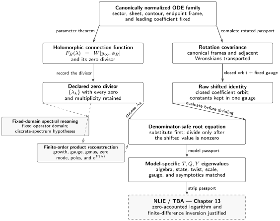
The ODE/IM dependency graph. The analytic/spectral branch supplies a connection divisor and, under stronger hypotheses, its operator meaning and product reconstruction. The covariance/Wronskian branch independently supplies the shifted identity. They meet at root evaluation. Naming the result $T$, $Q$, or $Y$ requires a model passport; logarithmic inversion requires a strip passport and belongs to Chapter 13.

Connection zeros become spectra only for a fixed domain

The geometric meaning of

$$F_B(\lambda_*)=0$$

is that the two declared solution lines coincide at $\lambda_*$. This is already a valid connection or resonance condition. It is an eigenvalue of a fixed operator $H_B$ only when those lines encode a $\lambda$-independent operator domain and

$$F_B(\lambda)=0 \quad\Longleftrightarrow\quad \lambda\in\sigma(H_B).$$

For the positive half-line oscillators of Page 1, the recessive line is the $L^2$ condition at infinity and Dirichlet or Neumann data at zero define fixed self-adjoint domains. Compact resolvent then gives a discrete spectrum, and Sturm–Liouville theory gives simple real zeros. Those conclusions do not follow from the Wronskian notation alone. On a complex contour, the positivity identity behind simplicity is no longer available: a bilinear self-overlap can vanish, and multiple zeros or exceptional points can occur.

A useful counterexample is an energy-dependent Robin condition,

$$u'(0)=h(\lambda)u(0).$$

Its characteristic function

$$F_h(\lambda) =y_\infty'(0,\lambda) -h(\lambda)y_\infty(0,\lambda)$$

may be entire, but if $h$ is nonconstant its zeros solve a nonlinear eigenparameter problem. They are not automatically the spectrum of one operator with a fixed domain in the original Hilbert space. Such problems can be linearized in a larger space in special cases, but that is additional structure.

Regular-singular endpoints add a second warning. If the exponent difference is resonant, a local basis can take the form

$$\phi_2 =\kappa\,\phi_1\log x +x^{r_2}\sum_{n\ge0}b_nx^n.$$

An integer exponent difference permits a logarithm but does not force one when the obstruction coefficient vanishes; coalesced exponents do force a logarithmic companion. The coefficient called “singular,” “regular,” or “alternate” depends on that normalization.

For the inverse-square coefficient, write

$$g=l(l+1)=m^2-\frac14, \qquad m=l+\frac12.$$

For real $l\ge-1/2$, the origin is limit-circle when $-1/2\le l<1/2$ and limit-point when $l\ge1/2$. A boundary condition is therefore required in the first range. At $l=-1/2$ the two modes coalesce into $x^{1/2}$ and $x^{1/2}\log x$; for $g<-1/4$ the operator defined minimally from $C_c^\infty(0,\infty)$ is not semibounded, so it has no Friedrichs extension. Analytic continuation in $l$ is useful connection theory, but it is not analytic continuation of one fixed self-adjoint domain.

A zero set is not yet a normalized determinant

Suppose $F$ is entire of finite order and its nonzero zeros $\{\lambda_n\}$ are known with multiplicity. Hadamard factorization has the form

$$\begin{aligned} F(\lambda) ={}& c\,\lambda^m\ee^{P(\lambda)} \prod_n \mathcal E_p\!\left(\frac{\lambda}{\lambda_n}\right). \end{aligned}$$

Here $c\in\mathbb C^\times$, the constant term has been absorbed so that $P(0)=0$, and

$$\begin{aligned} \mathcal E_0(w)&=1-w, \\ \mathcal E_p(w) &=(1-w) \exp\!\left( \sum_{j=1}^{p}\frac{w^j}{j} \right), \qquad p\ge1. \end{aligned}$$

The zeros do not specify the multiplicity $m$ at the origin, the polynomial $P$, the constant $c$, or any poles if the object is meromorphic. These data must come from growth and normalization.

The eigenvalue law fixes the exponent of convergence of the zero set and therefore only a lower bound on the order of an entire function having those zeros. Matching that exponent to the actual order requires a global ODE upper bound on the canonically normalized endpoint function; it does not follow from Weyl asymptotics alone.

For the homogeneous oscillator with $M>1$, Page 1 supplied both inputs and established order

$$\rho_M=\frac{M+1}{2M}<1.$$

The genus is zero and the order bound forces $P\equiv0$ in this convention; since $F(0)=1$, one also has $m=0$ and $c=1$. The zeros then determine

$$F(\lambda) =\prod_n\left(1-\frac{\lambda}{\lambda_n}\right).$$

At the harmonic threshold $M=1$, the order is one. If $F(0)=1$, then

$$F_c(\lambda)=\ee^{c\lambda}F(\lambda)$$

has the same zeros, the same value at zero, and the same order for every $c\in\mathbb C$. A derivative, zeta prescription, canonical asymptotic, or another normalization condition must fix $c$.

The canonical product and a zeta-normalized determinant are also different normalizations. With the sign convention appropriate to $H-\lambda$, write $\Delta_p$ for the genus-$p$ product. Below order one, the comparison can take the form

$$D_\zeta(\lambda) =D_\zeta(0)\Delta_0(\lambda), \qquad D_\zeta(0)=\ee^{-Z'(0)}.$$

At order one the general comparison retains the linear zero-free factor,

$$D_\zeta(\lambda) =D_\zeta(0)\ee^{a\lambda}\Delta_1(\lambda),$$

where $a$ is fixed by the zeta prescription. The signs inside the products reverse for the $H+\lambda$ convention. Here $Z$ is the continued spectral zeta function; for a complex spectrum, its spectral cut and continuation prescription must be declared. Equality between either object and a canonically normalized endpoint value is a comparison theorem, not a consequence of sharing zeros. The corrigendum to Voros’s 1999 paper is essential when the logarithmic WKB coefficient is nonzero.

Zero-energy normalization can fail even below order one. If $F(\lambda)$ has a zero of order $m$ at $\lambda=0$, write

$$F(\lambda) =c_m\lambda^m\widetilde F(\lambda), \qquad c_m=\frac{F^{(m)}(0)}{m!}, \qquad \widetilde F(0)=1.$$

Dividing by $F(0)$ is meaningless. The zero mode must be extracted before forming a normalized determinant or a logarithmic derivative.

Raw Wronskian identities survive gauge changes; their constants do not

Linear dependence and the Plücker identity are algebraic. Once the solution representatives are fixed, their Wronskian identities are exact. For the Page 7 deformation,

$$\begin{aligned} T_\sigma(E)D_\sigma(E) ={}& \omega^{-\kappa_\sigma} D_{-\sigma}(\omega^{-2}E) \\ &+ \omega^{\kappa_\sigma} D_{-\sigma}(\omega^2E) \end{aligned}$$

is a raw connection identity. Provided $D_\sigma(0)D_{-\sigma}(0)\ne0$, independently setting $\widehat D_\sigma=D_\sigma/D_\sigma(0)$ introduces the factor

$$r_\sigma=\frac{D_{-\sigma}(0)}{D_\sigma(0)}.$$

Dropping $r_\sigma$ changes the equation.

More generally, a zero-free change

$$D_j(\lambda)\longmapsto h_j(\lambda)D_j(\lambda)$$

does not move zeros but changes shifted coefficients unless the $h_j$ obey a compatible difference equation. This is why a Stokes gauge, a determinant normalized at zero, and an operator $Q$-eigenvalue cannot be exchanged by notation alone.

The generalized Mathieu relation on Page 7 gives a numerical audit. In the source gauge,

$$1+Q_1Q_2=Q_3Q_0.$$

Multiplying both canonical families by $\sqrt2$ gives $\widehat Q=2Q$, so the same identity becomes

$$4+\widehat Q_1\widehat Q_2 =\widehat Q_3\widehat Q_0.$$

The constant is part of the Wronskian normalization, not a universal property of the printed letters.

Evaluate at a zero before dividing

Let a shifted relation have the local form

$$T(\lambda)D(\lambda) =a\,G(q^{-2}\lambda) +b\,G(q^2\lambda), \qquad ab\ne0.$$

Assume here that $T$, $a$, $b$, and the two shifted values of $G$ are finite at the chosen zero. This is automatic for the entire TQ systems used earlier in the chapter, but not for a merely meromorphic identity. If $T$ has a pole that cancels the zero of $D$, then $TD$ need not vanish; one must first clear the poles or take the regularized limit.

At a zero $\lambda_k$ of $D$, the always-valid statement is

$$a\,G(q^{-2}\lambda_k) +b\,G(q^2\lambda_k)=0.$$

Only if

$$G(q^{-2}\lambda_k)\ne0$$

may one write

$$\frac{G(q^2\lambda_k)} {G(q^{-2}\lambda_k)} =-\frac{a}{b}.$$

If both shifted values vanish, the denominator-free equation reduces to $0=0$ and supplies no ratio. Such a collision requires additional divisor data—for example a $q^4$-related pair of zeros or an exact zero string—and must be checked rather than inferred from resonance alone. When present, it must be resolved by a limiting equation, a derivative identity, or a different functional relation.

Substituting an infinite product is a second, independent step. If

$$G(\lambda) =\lambda^m\ee^{P(\lambda)} \prod_n \mathcal E_p\!\left(\frac{\lambda}{\mu_n}\right),$$

then, for $\lambda\ne0$, the complete shifted ratio is

$$\begin{aligned} \frac{G(q^2\lambda)}{G(q^{-2}\lambda)} ={}&q^{4m} \exp\!\left[ P(q^2\lambda)-P(q^{-2}\lambda) \right] \\ &\times \prod_n \frac{\mathcal E_p(q^2\lambda/\mu_n)} {\mathcal E_p(q^{-2}\lambda/\mu_n)}. \end{aligned}$$

The factor $q^{4m}$ records a zero at the normalization point. At $\lambda=0$ with $m>0$, both shifted values vanish and the ratio is $0/0$ until that zero mode is extracted. The $P$-factor cancels in the genus-zero, constant-$P$ situation used on Pages 4–7; it need not cancel at order one. A product Bethe equation is therefore not obtained from a zero set alone.

ODE closure does not identify an integrable model

An ODE can produce a function satisfying a TQ-shaped equation without producing a Baxter operator. The following dictionary is the minimum needed to promote analogy to identification:

Printed object	Additional evidence required
Spectral determinant	Fixed boundary domain, compact or controlled resolvent, zero multiplicities, growth, and normalization
Baxter $Q$	Named model and algebra, representation or state, spectral scale, twist, normalization, and matching analytic class
Transfer function $T$	A specified Stokes multiplier plus the transfer-matrix dictionary and fusion convention
Bethe roots	Root identification, admissibility, completeness or a stated restricted sector, and treatment of exceptional roots
$Y$-function	A declared combination of $T$ or $Q$ functions, shift convention, and analytic strip

The generic polynomial orbit of Page 7 illustrates the distinction. Covariance yields a finite vector of determinants belonging to conjugate complex-scaled operators. That is an exact ODE system. It is not automatically the spectrum of one Baxter operator. Conversely, the massive sine–/sinh–Gordon correspondence starts from an auxiliary linear system over a specified nonlinear background, not from an arbitrary scalar exponential potential.

The BLZ normalization supplies another branch warning. In their convention,

$$\mathbf Q_\pm(\lambda) =\lambda^{\pm2P/\beta^2}\mathbf A_\pm(\lambda),$$

so a highest-weight matrix element of raw $\mathbf Q_\pm$ contains a momentum-dependent monomial and can be multivalued at the origin. Away from the resonance lattice below, the stripped vacuum functions obey $A_\pm(0,p)=1$. For $0<\beta^2<1/2$, BLZ III proves their entirety in $\lambda^2$ for all rational $\beta^2$ and almost every irrational $\beta^2$, subject to

$$2p\ne n\beta^2+m, \qquad n\in\mathbb Z_{>0}, \quad m\in\mathbb Z.$$

Extension to the exceptional measure-zero set of irrational values is assumed there, not proved. It is this stripped, single-valued object in its established parameter range—not every raw quantity printed with the letter $Q$—that Pages 4–6 compare with the ODE determinants.

Even within a named model, functional equations need not determine a unique eigenvalue. State selection enters through asymptotics, zero locations, reality, periodicity, and normalization. Dorey–Dunning–Tateo and Bazhanov–Lukyanov–Zamolodchikov make such analytic assumptions explicit when passing from Baxter relations to nonlinear integral equations.

Exact functional system, conditional inversion

For the Page 7 $\pm\alpha$ family, Dorey–Dunning–Tateo suppose before their NLIE derivation that all determinant zeros lie on the positive real $E$-axis and all relevant transfer-function zeros lie off that axis. The TQ relations alone do not prove these locations. The paper also notes that a rigorous uniqueness proof for the iterated NLIE is not available in the stated regime, while the direct Bethe equations outside it admit multiple branches unless quantum numbers and asymptotics are supplied. At quasi-exactly solvable points, the paper establishes coincidences between certain determinant and transfer-function zeros. A $0/0$ determinant ratio follows only when an additional $q^4$-related shifted determinant zero is present; the QES coincidence alone does not prove that stronger condition.

A functional relation is not yet a TBA equation

Suppose a $Y$-system is known in a strip,

$$Y(\theta+\ii\eta)Y(\theta-\ii\eta) =\mathcal F(Y(\theta)).$$

Writing an additive equation for $\log Y$ requires a continuous branch. The right-hand side also requires a branch of its logarithm; schematically,

$$\begin{aligned} \log Y(\theta+\ii\eta) &+\log Y(\theta-\ii\eta) \\ &=\log\mathcal F(Y(\theta))+2\pi\ii N. \end{aligned}$$

The locally constant integer $N$ is fixed only after branch and asymptotic data are chosen. Zeros or poles of $Y$, and zeros or poles of $\mathcal F(Y)$, including zeros of factors such as $1+Y$, create logarithmic singularities and, after contour displacement, explicit source terms. Fourier inversion also needs large-$|\Re\theta|$ asymptotics to identify the driving term, decay or subtractions to control boundary terms, and a prescription for homogeneous modes whenever the chosen finite-difference operator has a kernel in the admitted analytic class.

These inputs are uniqueness data. A periodic or zero-free homogeneous factor can preserve a functional relation while changing its asymptotics and logarithm. Therefore the equation by itself does not select a ground state, an excited state, or even a unique analytic solution.

Chapter 13 begins from precisely this point. It will declare the analytic strip, derive the convolution kernel, compute the driving term, track zeros and poles through contour deformations, and estimate the error of numerical iteration. No such inversion is asserted on this page.

A reproducible correspondence audit

Before using a proposed ODE/IM formula, audit its dependency graph branch by branch:

1. Common analytic base: record the spectral coordinate, cover, deleted divisors, canonical representatives, logarithmic powers, sectors, contours, and the theorem that makes each solution or Wronskian holomorphic, entire, or meromorphic.
2. Covariance branch: transport the complete ODE passport, verify orbit closure, and derive the raw shifted identity before changing any Wronskian or determinant gauge.
3. Spectral and factorization branch: distinguish the connection divisor from a fixed operator domain; then establish order, genus, zero multiplicities, poles, zero modes, and every zero-free exponential factor.
4. Root-evaluation merge: substitute the zero into the raw identity first, retain the denominator-free equation, and state each shifted nonvanishing assumption used in a ratio or product form.
5. Model passport: name the algebra, model, representation or state, twist, spectral scale, normalization, and matching analytic class and asymptotics.
6. Inversion passport: declare the strip, zeros and poles of every logarithm argument, integer branch constants, driving asymptotic, contour, subtractions, and any homogeneous modes admitted by the chosen difference operator.

A missing gate blocks only claims downstream on that branch; independent ODE identities retain their stated scope. Stopping there is the correct mathematical result, not a failure of the method.

Common pitfalls

Using “analytic” without a domain. Holomorphy on a slit plane, entirety in $E$, and a zero-free rapidity strip are different claims. Write the variable and domain every time the distinction matters.

Calling a connection zero an eigenvalue. The zero only says that two solution lines coincide. A fixed closed operator domain is extra data.

Reconstructing from zeros at order one. The factor $\ee^{c\lambda}$ survives both the zero set and the condition $F(0)=1$. Growth type or another normalization must fix it.

Dividing the root equation too early. Keep the linear, denominator-free relation until the shifted denominator is proved nonzero.

Deriving TBA from algebra alone. Logarithm branches, strip singularities, asymptotics, and contour terms carry physical state data. Ignoring them can turn a valid functional relation into the wrong integral equation.

Exercises

1. Type three analyticity claims. Classify

$$f(\lambda)=\sqrt{\lambda}, \qquad g(\theta)=\sin\theta, \qquad h(\lambda)=\frac{1}{1-\lambda}$$

as holomorphic on a domain or cover, entire, meromorphic, and locally logarithmable. State the missing domain data in each case.

Solution

The square root is holomorphic after a branch is chosen on a slit plane, or globally on the two-fold cover of $\mathbb C^\times$. It is not an entire single-valued function of the coordinate $\lambda$ because zero is a branch point. It has a holomorphic logarithm only on a simply connected subdomain avoiding its zero and the chosen cut.

The sine function is entire in $\theta$, but its zeros at $\theta=n\pi$ prevent a global holomorphic logarithm. On any simply connected domain avoiding those zeros, a branch of $\log\sin\theta$ exists.

The rational function $h$ is holomorphic on $\mathbb C\setminus\{1\}$ and meromorphic on $\mathbb C$, with one pole at $\lambda=1$. It has a local logarithm on every sufficiently small disk avoiding its pole and its zero set; since it has no finite zeros, the only local obstruction is the pole. Thus “all three are analytic” would hide three different parameter passports.

2. Detect a moving boundary problem. Let $y_\infty(x,\lambda)$ be the solution of

$$\left[-\frac{\dd^2}{\dd x^2}+x^2\right]y =\lambda y$$

that is recessive as $x\to+\infty$. Compare

$$\begin{aligned} F_{h_0}(\lambda) &=y_\infty'(0,\lambda)-h_0y_\infty(0,\lambda), \\ F_{\mathrm{mov}}(\lambda) &=y_\infty'(0,\lambda)-\lambda y_\infty(0,\lambda). \end{aligned}$$

Why does only the first immediately describe a fixed Robin realization?

Solution

A zero of $F_{h_0}$ satisfies

$$u'(0)=h_0u(0),$$

where $h_0$ is fixed independently of the spectral parameter. Together with recession at infinity this is the eigenvalue condition for one closed half-line Robin operator.

A zero of $F_{\mathrm{mov}}$ instead satisfies

$$u'(0)=\lambda u(0).$$

The boundary line changes with the value being solved for, so there is no single domain $\{u:u'(0)=\lambda u(0)\}$ independent of $\lambda$. The zeros remain perfectly valid connection data for an eigenparameter-dependent boundary problem. Calling them the spectrum of one ordinary Schrödinger operator would require a separate linearization or enlarged-space construction.

3. Exhibit the order-one ambiguity. Let $\{\lambda_n\}$ have exponent of convergence one and let

$$P(\lambda) =\prod_n \mathcal E_1\!\left(\frac{\lambda}{\lambda_n}\right), \qquad P(0)=1.$$

Show that the zeros and the value at zero do not determine an order-one entire function. Which one additional scalar datum fixes the ambiguity within the family below?

Solution

For every $c\in\mathbb C$,

$$F_c(\lambda)=\ee^{c\lambda}P(\lambda)$$

is entire of order at most one, has the same zeros with the same multiplicities, and obeys $F_c(0)=1$. Hence the zeros and zero-energy normalization leave $c$ undetermined.

The logarithmic derivative at zero fixes it:

$$c = \left.\frac{\dd}{\dd\lambda}\log F_c(\lambda) \right|_{\lambda=0} - \left.\frac{\dd}{\dd\lambda}\log P(\lambda) \right|_{\lambda=0}.$$

Equivalent choices include the complex coefficient of $\lambda$ in a specified logarithmic asymptotic or a zeta-regularized logarithmic derivative at zero. This is the ambiguity met at the harmonic threshold.

4. Remove a zero mode before normalizing. Suppose $F$ is entire and has a zero of exact order $m\ge1$ at the origin. Construct a function $\widetilde F$ with $\widetilde F(0)=1$ and separate the singular part of its logarithmic derivative.

Solution

Taylor’s theorem gives

$$F(\lambda) = \frac{F^{(m)}(0)}{m!}\lambda^m +O(\lambda^{m+1}).$$

Therefore define

$$\widetilde F(\lambda) = \frac{m!\,F(\lambda)} {F^{(m)}(0)\lambda^m}.$$

The apparent singularity is removable and $\widetilde F(0)=1$. Moreover,

$$\frac{F'(\lambda)}{F(\lambda)} = \frac{m}{\lambda} +\frac{\widetilde F'(\lambda)} {\widetilde F(\lambda)}.$$

The first term is the explicit zero-mode contribution. Any trace or TBA formula using the logarithmic derivative must retain or subtract it deliberately.

5. Transport a shifted identity through two gauges. Starting from

$$T(\lambda)D(\lambda) =a(\lambda)G(q^{-2}\lambda) +b(\lambda)G(q^2\lambda),$$

set $\widehat D=hD$ and $\widehat G=gG$, where $h$ and $g$ are entire and nowhere zero, and assume $a(\lambda)b(\lambda)\ne0$ on the domain being audited. Derive the transformed coefficients. Which compatibility conditions preserve the printed coefficients $a$ and $b$ when $T$ itself is unchanged?

Solution

Substitution gives

$$\begin{aligned} T(\lambda)\widehat D(\lambda) ={}&a(\lambda) \frac{h(\lambda)}{g(q^{-2}\lambda)} \widehat G(q^{-2}\lambda) \\ &+b(\lambda) \frac{h(\lambda)}{g(q^2\lambda)} \widehat G(q^2\lambda). \end{aligned}$$

Thus the displayed coefficients are preserved precisely when

$$h(\lambda) =g(q^{-2}\lambda) =g(q^2\lambda)$$

on the domain in question. The gauges preserve the zero divisors but generically alter both shifted coefficients. If $D=G$ and $h=g$, even the seemingly harmless change $D\mapsto hD$ must satisfy a restrictive difference symmetry before the old TQ equation can be reused verbatim.

6. Audit a collision of labelled roots. Consider

$$F(\lambda,p)=\lambda^2-p.$$

Show that $F$ is jointly entire while its two labelled roots are not single-valued near $p=0$. Determine the multiplicity at the collision and explain what fails in a naïve continuation of one Bethe root.

Solution

The polynomial is entire on $\mathbb C^2$. For $p\ne0$ its roots are

$$\lambda_\pm(p)=\pm\sqrt p.$$

A circuit around $p=0$ exchanges the two labels, so neither root is a single-valued holomorphic function on a punctured neighborhood of the collision. At $p=0$,

$$F(\lambda,0)=\lambda^2, \qquad \partial_\lambda F(0,0)=0,$$

so the zero has multiplicity two and the implicit-function theorem does not provide a local root label. The divisor and its symmetric data remain single-valued—for example, the root sum is zero and the product is $-p$—but a naïve Bethe-root continuation depends on a chosen sheet and is permuted by monodromy. Any argument differentiating a labelled root through $p=0$ must instead use the full divisor or a uniformizing coordinate.

7. Find the missing factors in an order-one Bethe product. Let

$$G(\lambda) =\ee^{c\lambda} \prod_n\mathcal E_1\!\left(\frac{\lambda}{\mu_n}\right),$$

where the genus-one canonical product converges. Compute $G(q^2\lambda)/G(q^{-2}\lambda)$ and identify the data that a bare zero set does not supply.

Solution

Direct substitution gives

$$\begin{aligned} \frac{G(q^2\lambda)} {G(q^{-2}\lambda)} ={}& \ee^{c(q^2-q^{-2})\lambda} \\ &\times \prod_n \frac{1-q^2\lambda/\mu_n} {1-q^{-2}\lambda/\mu_n} \exp\!\left[ \frac{(q^2-q^{-2})\lambda}{\mu_n} \right]. \end{aligned}$$

The canonical convergence exponentials are part of the genus-one product, while the separate zero-free factor contains the undetermined constant $c$. Neither may be discarded term by term. The latter disappears only when $c=0$, when $q^2=q^{-2}$ in a degenerate case, or when another normalization identity cancels it. Thus an order-one root equation cannot be inferred from the zeros as if the determinant had genus zero.

8. Explain why a $Y$-system does not fix its TBA. Assume

$$Y(\theta+\ii\eta)Y(\theta-\ii\eta) =1+Y(\theta).$$

List the data required to Fourier-invert its logarithm. Explain the effect of a simple zero of $Y$ inside the intended strip.

Solution

One must specify a strip wide enough for both shifted contours, all zeros and poles of $Y$ in that strip, all zeros of $1+Y$, continuous branches of both logarithms away from them, the integer $2\pi\ii N$ relating the chosen branches, large-$|\Re\theta|$ asymptotics, any necessary subtraction, decay of the transformed remainder, and the treatment of homogeneous modes if the selected difference operator has a kernel in the admitted analytic class. These data determine the driving term and the allowed contour displacement.

If $Y(\theta_0)=0$ simply, then locally

$$\log Y(\theta) =\log(\theta-\theta_0)+O(1).$$

Moving a shifted contour past $\theta_0$ picks up a logarithmic source term. Omitting it gives an integral equation for a different analytic state even though the printed $Y$-system is unchanged. Chapter 13 turns this observation into the ground-state and excited-state contour prescriptions.

References

• P.-F. Hsieh and Y. Sibuya, “On the Asymptotic Integration of Second Order Linear Ordinary Differential Equations with Polynomial Coefficients”, Journal of Mathematical Analysis and Applications 16 (1966), 84–103, for canonical recessive solutions with analytic parameter dependence.
• H. E. Gollwitzer and Y. Sibuya, “Stokes Multipliers for Subdominant Solutions of Second Order Differential Equations with Polynomial Coefficients”, Journal für die reine und angewandte Mathematik 243 (1970), 98–119, for parameter-entire Stokes multipliers in the fixed polynomial family.
• Y. Sibuya, Global Theory of a Second Order Linear Ordinary Differential Equation with a Polynomial Coefficient, North-Holland Mathematics Studies 18, 1975, for global polynomial Stokes geometry and canonical parameter-entire solutions.
• B. Ya. Levin, Distribution of Zeros of Entire Functions, Translations of Mathematical Monographs 5, AMS, 1964, for order, exponent of convergence, canonical products, and Hadamard factorization.
• A. Voros, “Exact Resolution Method for General 1D Polynomial Schrödinger Equation”, Journal of Physics A 32 (1999), 5993–6007, with corrigendum, 33 (2000), 5783–5784, for rotated polynomial operators, determinant normalizations, and exact quantization conditions.
• P. Dorey, C. Dunning, and R. Tateo, “Spectral Equivalences, Bethe Ansatz Equations, and Reality Properties in PT-Symmetric Quantum Mechanics”, Journal of Physics A 34 (2001), 5679–5704, for the coupled determinant system and the root-location assumptions entering its nonlinear integral equations.
• P. Dorey, C. Dunning, and R. Tateo, “The ODE/IM Correspondence”, Journal of Physics A 40 (2007), R205–R283, for the scope of polynomial ODE analyticity, determinant products, Bethe equations, and ODE/IM dictionaries.
• V. V. Bazhanov, S. L. Lukyanov, and A. B. Zamolodchikov, “Integrable Structure of Conformal Field Theory II. Q-Operator and DDV Equation”, Communications in Mathematical Physics 190 (1997), 247–278, for the operator $Q$ construction and the analytic assumptions needed to pass from Baxter relations to a nonlinear integral equation.
• V. V. Bazhanov, S. L. Lukyanov, and A. B. Zamolodchikov, “Integrable Structure of Conformal Field Theory III. The Yang–Baxter Relation”, Communications in Mathematical Physics 200 (1999), 297–324, for the proven and exceptional parameter ranges in the analyticity of transfer and stripped $Q$-functions.
• NIST Digital Library of Mathematical Functions, Fuchs–Frobenius theory, for resonant regular-singular points and logarithmic local solutions.
• J. Dereziński and S. Richard, “On Schrödinger Operators with Inverse Square Potentials on the Half-Line”, Annales Henri Poincaré 18 (2017), 869–928, for limit-point and limit-circle domains, homogeneous extensions, and the coalesced logarithmic case.
• G. Teschl, Mathematical Methods in Quantum Mechanics, second edition, AMS, 2014, for fixed self-adjoint realizations, boundary conditions, compact resolvents, and one-dimensional spectral theory.