Verified Numerics: Conditioning, Precision, and Independent Checks

A long decimal expansion is an output format, not a theorem. A continued fraction can converge to the wrong branch; two implementations can agree because they share the same incorrect recurrence; a tiny residual can lie deep inside a nonnormal pseudospectrum; and a ball enclosing a zero of a finite determinant proves nothing yet about the infinite recurrence.

This page turns the direct methods of the chapter into an evidence architecture. Its central principle is simple:

A numerical claim is only as strong as the largest error source that has actually been bounded.

The beginner’s practical task is to vary cutoff and precision separately, report scales, and compare a genuinely different representation. The expert’s additional task is to replace observed differences by outward-rounded enclosures and a root-count or inclusion theorem. A Bessel disk problem will show every level, from a floating candidate to an exact rational certificate.

First pass through the page

Read the evidence table, the three-term error identity, the cutoff–tail-order–precision grid, the Bessel laboratory, and the reproduction manifest. Return to nonlinear-pencil conditioning, rigorous tail balls, Rouché, and Krawczyk inclusion when you need proof rather than a convergence audit.

Numerical evidence has two axes

The words converged, verified, and certified should not be used interchangeably. We will attach the following meanings to them.

Claim	Minimum evidence
Computed	One declared algorithm returns a candidate
Internally converged	The candidate is stable on a cutoff, tail-order, precision, and chart-refinement grid
Cross-verified	A representation with substantially different failure modes agrees under its own refinements
Certified	Outward-rounded bounds plus a theorem enclose a root or prove a root count for the declared mathematical problem
Physically validated	The equation, domain, boundary conditions, normalization, branches, and sheet represent the intended physical observable

These are not quite a single ladder. Certification concerns a mathematical model; physical validation concerns whether that model is the right one. A rigorously enclosed eigenvalue of the wrong boundary problem is certified and physically irrelevant. Conversely, a well-motivated QNM computed by two excellent codes may be physically persuasive but still not mathematically certified.

The book-wide status convention reserves “certified” for theorem-backed enclosures. Ordinary high-precision agreement will be called cross-verification.

One identity exposes three numerical errors

Let $F(\lambda)$ be an exact analytic characteristic function on the chosen sheet. It might be an Abel-normalized Wronskian, a homogeneous Casoratian, or an analytic determinant. Let

$$F_N(\lambda)$$

be a finite-cutoff approximation and let

$$\widehat F_{N,p}(\lambda)$$

be its floating-point evaluation at $p$ decimal digits of working precision. If the root solver returns $\widehat\lambda$, the exact identity

$$\begin{aligned} F(\widehat\lambda) ={}& \bigl[F-F_N\bigr](\widehat\lambda) \\ &+ \bigl[F_N-\widehat F_{N,p}\bigr](\widehat\lambda) \\ &+ \widehat F_{N,p}(\widehat\lambda) \end{aligned}$$

separates:

1. tail or discretization error, from replacing the infinite problem by $F_N$;
2. evaluation error, including rounding, cancellation, and inexact coefficients;
3. nonlinear-solve residual, left by the root finder.

Consequently, proved bounds

$$\begin{aligned} \left|F-F_N\right| &\leq\varepsilon_{\mathrm{tail}}, \\ \left|F_N-\widehat F_{N,p}\right| &\leq\varepsilon_{\mathrm{eval}}, \\ \left|\widehat F_{N,p}(\widehat\lambda)\right| &\leq\varepsilon_{\mathrm{solve}} \end{aligned}$$

give a function-value bound

$$\left|F(\widehat\lambda)\right| \leq \varepsilon_{\mathrm{tail}} + \varepsilon_{\mathrm{eval}} + \varepsilon_{\mathrm{solve}}.$$

This is not yet a root-error bound. That conversion is a conditioning problem.

There is also a fourth category that the identity cannot see: model and dictionary error. A wrong sign in the recurrence, a mistaken Fourier convention, a frozen angular eigenvalue, or a sheet mismatch changes the exact $F$ itself. More precision merely computes the wrong object more accurately.

The first omitted row belongs to the residual

A finite recurrence can have zero residual in every retained row while failing badly as a vector of the infinite operator. If

$$\alpha_nu_{n+1} +\beta_nu_n +\gamma_nu_{n-1} =0$$

is truncated after $u_N$ and the vector is extended by zeros, the first discarded row is

$$r_{N+1} = \gamma_{N+1}u_N.$$

It must be included in the full residual norm. A vanishing finite determinant or retained-row residual does not make this term disappear.

For a self-adjoint operator $A$ and a normalized vector $u$,

$$\operatorname{dist} \bigl( \widehat\lambda,\sigma(A) \bigr) \leq \left\| (A-\widehat\lambda)u \right\|.$$

Even there, the conclusion is only that some spectral point is nearby. A spectral gap or an oscillation theorem is needed to identify an isolated eigenvalue; the closest point may instead belong to continuous spectrum. For a nonnormal operator, the corresponding residual statement is pseudospectral and can be dramatically weaker.

Backward error is not forward error

Suppose $\lambda_*$ is a simple zero of a scalar characteristic function:

$$F(\lambda_*)=0, \qquad F'(\lambda_*)\neq0.$$

For a precise first-order statement, let

$$F_t=F+tG+O(t^2)$$

in a local holomorphic norm. The implicit-function theorem gives a root $\lambda(t)$ with

$$\lambda(t) = \lambda_* - \frac{ tG(\lambda_*) }{ F'(\lambda_*) } + O(t^2).$$

Thus $\delta\lambda=-\delta F(\lambda_*)/F'(\lambda_*)$ to first order. A pointwise residual alone is not a finite-error theorem; the local perturbation family or a disk enclosure controls the remainder. The numerator also needs a declared scale. If the perturbation model is

$$\left|\delta F(\lambda_*)\right| \leq \varepsilon S_F(\lambda_*),$$

define

$$\kappa_{\mathrm{abs}} = \frac{ S_F(\lambda_*) }{ \left|F'(\lambda_*)\right| },$$

and, when $\lambda_*\neq0$,

$$\kappa_{\mathrm{rel}} = \frac{ S_F(\lambda_*) }{ |\lambda_*| \left|F'(\lambda_*)\right| }.$$

The scale $S_F$ is part of the result. Quoting $1/|F'(\lambda_*)|$ without a normalization or perturbation model is not invariant.

The Newton correction

$$\beta(\widehat\lambda) = \left| \frac{ F(\widehat\lambda) }{ F'(\widehat\lambda) } \right|$$

is an excellent local diagnostic when the zero is simple, the iterate is already in its local basin, $F$ and $F'$ are evaluated more accurately than the claimed correction, and no ratio-chart pole lies nearby. It is not by itself a certified error bound.

If the root has multiplicity $m$, a generic perturbation instead produces

$$|\delta\lambda| = O\left(\varepsilon^{1/m}\right).$$

The ordinary derivative condition number is then infinite. A double root can require roughly twice as many residual digits as desired root digits, and ordinary Newton iteration loses its quadratic behavior.

Wronskian scales make matching diagnostics meaningful

For two solution jets at a common match point, write

$$x= \begin{pmatrix} f\\ f' \end{pmatrix}, \qquad y= \begin{pmatrix} g\\ g' \end{pmatrix}, \qquad F=\det(x,y).$$

Let

$$S_W=\|x\|_2\|y\|_2.$$

If

$$\|\delta x\|_2\leq\varepsilon_x\|x\|_2, \qquad \|\delta y\|_2\leq\varepsilon_y\|y\|_2,$$

bilinearity of the determinant and $|\det(a,b)|\leq\|a\|_2\|b\|_2$ give the exact perturbation bound

$$|\delta F| \leq \left( \varepsilon_x + \varepsilon_y + \varepsilon_x\varepsilon_y \right) S_W.$$

At a simple matching zero, the natural absolute condition scale is therefore

$$\kappa_{\mathrm{match}} = \frac{ S_W(\lambda_*) }{ |F'(\lambda_*)| }.$$

With

$$\varepsilon_W = \varepsilon_x + \varepsilon_y + \varepsilon_x\varepsilon_y,$$

the first-order root estimate is

$$|\delta\lambda| \lesssim \kappa_{\mathrm{match}}\varepsilon_W.$$

If both jet errors are bounded by the same $\varepsilon$, the leading coefficient is $2\kappa_{\mathrm{match}}\varepsilon$, not $\kappa_{\mathrm{match}}\varepsilon$.

At the zero this ratio is unchanged if the two jets are separately multiplied by nonzero analytic factors. Indeed, both $S_W$ and $|F'|$ acquire the same factor. It still depends on the spectral coordinate, ODE gauge, jet norm, and coordinate derivative used to form the jets; those choices belong in the report.

Away from a zero,

$$\kappa_{\mathrm{eval},W} = \frac{ |fg'|+|f'g| }{ |fg'-f'g| }$$

measures cancellation in the two-term determinant evaluation. Its divergence near a genuine zero is expected. Use the analytic $F$ in Newton iteration; the nonholomorphic quantity $|F|/S_W$ is a reporting diagnostic, not a replacement characteristic function.

Parameter derivatives should come from variational equations. If

$$Y'=A(z,\lambda)Y,$$

then

$$\left(\partial_\lambda Y\right)' = A\,\partial_\lambda Y + A_\lambda Y.$$

For a Wronskian condition,

$$F' = \operatorname{Wr} \left[ \partial_\lambda f,g \right] + \operatorname{Wr} \left[ f,\partial_\lambda g \right].$$

This avoids a finite-difference step that can cross a branch cut, amplify cancellation, or silently hold an asymptotic endpoint seed fixed.

Left and right eigenvectors reveal nonnormal sensitivity

For an analytic matrix function

$$T(\lambda) = \sum_{j=1}^{s} f_j(\lambda)A_j,$$

declare unstructured coefficient perturbations

$$\|\Delta A_j\|_2 \leq \varepsilon\omega_j$$

and set

$$s_\omega(\lambda) = \sum_{j=1}^{s} \omega_j|f_j(\lambda)|.$$

For an approximate eigenpair $(\widehat\lambda,\widehat v)$, the normwise backward error is

$$\eta(\widehat\lambda,\widehat v) = \frac{ \|T(\widehat\lambda)\widehat v\|_2 }{ s_\omega(\widehat\lambda) \|\widehat v\|_2 }.$$

Minimizing over $\widehat v$ gives

$$\eta(\widehat\lambda) = \frac{ \sigma_{\min}\!\left(T(\widehat\lambda)\right) }{ s_\omega(\widehat\lambda) }.$$

If $T(\lambda_*)v=0$ and $w^*T(\lambda_*)=0$ for a simple eigenvalue, then

$$\kappa_{\mathrm{abs}}(\lambda_*) = \frac{ s_\omega(\lambda_*) \|v\|_2\|w\|_2 }{ \left|w^*T'(\lambda_*)v\right| }.$$

To first order, forward error is condition number times backward error. A tridiagonal, symmetry-preserving, or physical-parameter perturbation model has a different structured condition number; the weights and structure must be declared.

An exact nonnormal warning

Let

$$A_\varepsilon = \begin{pmatrix} 1&1\\ \varepsilon^2&1 \end{pmatrix}, \qquad 0<\varepsilon\ll1.$$

Its eigenvalues and convenient right and left eigenvectors are

$$\begin{aligned} \lambda_\pm&=1\pm\varepsilon, \\ v_\pm&= \begin{pmatrix} 1\\ \pm\varepsilon \end{pmatrix}, \\ w_\pm&= \begin{pmatrix} \pm\varepsilon\\ 1 \end{pmatrix}. \end{aligned}$$

For the linear pencil $T=A_\varepsilon-\lambda I$, perturb only $A_\varepsilon$ and regard the coefficient of $-\lambda I$ as exact. Then

$$\kappa_{\mathrm{abs}}(\lambda_\pm) = \frac{ 1+\varepsilon^2 }{ 2\varepsilon }.$$

At the midpoint $\widehat\lambda=1$,

$$\left(A_\varepsilon-I\right)e_1 = \begin{pmatrix} 0\\ \varepsilon^2 \end{pmatrix}.$$

The residual is $\varepsilon^2$, while the nearest eigenvalue is distance $\varepsilon$. With $\varepsilon=10^{-30}$, a residual of $10^{-60}$ coexists with a forward error of $10^{-30}$. The small residual says that $1$ lies in a small pseudospectrum; it does not promise a comparably nearby eigenvalue.

Never use $|\det T(\widehat\lambda)|$ as a backward error. A determinant is strongly affected by dimension and row scaling and may be tiny because unrelated singular values are small.

Precision must be budgeted against lost digits

Suppose $t$ reliable relative digits are desired. A useful first scheduling estimate is

$$p_{\mathrm{work}} \gtrsim t + d_{\mathrm{cond}} + d_{\mathrm{eval}} + g,$$

where

$$d_{\mathrm{cond}} = \max\left( 0, \left\lceil \log_{10}\kappa_{\mathrm{rel}} \right\rceil \right),$$

$d_{\mathrm{eval}}$ estimates cancellation and growth inside the evaluator, and $g$ is a guard allowance. This is a resource estimate, not a proof. Tail error and uncertainty in the input coefficients remain separate.

Three rules prevent common precision illusions:

• Convert requested decimal digits to bits with an explicit guard; do not confuse a library’s bit precision with decimal digits.
• Parse exact inputs as integers, rationals, or decimal strings. Promoting a binary64 input to 200-digit arithmetic does not recover its missing digits.
• Increase precision until the evaluated function and derivative are more accurate than the claimed Newton correction. Increasing only the display precision changes nothing.

Use a cutoff–tail-order–precision grid

Write a candidate as

$$\lambda_{N,K,p,m},$$

where $N$ is the cutoff, $K$ the asymptotic tail order, $p$ the working precision, and $m$ a split index or match point. Then monitor, for example,

$$\begin{aligned} d_N &= \left| \lambda_{2N,K,p,m} - \lambda_{N,K,p,m} \right|, \\ d_K &= \left| \lambda_{N,K+1,p,m} - \lambda_{N,K,p,m} \right|, \\ d_p &= \left| \lambda_{N,K,p+\Delta p,m} - \lambda_{N,K,p,m} \right|. \end{aligned}$$

These are diagnostics, not bounds, until a convergence theorem controls the unseen remainder.

Axis varied	Hold fixed	What the comparison can expose
Cutoff $N$	High $p$, fixed $K$	Tail or discretization regime
Tail order $K$	$N$ and $p$	Quality and asymptotic consistency of the terminal seed
Precision $p$	$N$, $K$	Rounding plateau, cancellation, or an upturn
Split or match point $m$	$N$, $K$, $p$	Ratio-chart failure, propagation instability, or bad overlap
Spectral chart or uniformizer	Mathematical problem	Hidden poles, branch mistakes, and threshold nonuniformity

The trustworthy region is usually a two-dimensional knee: the tail error has fallen below the target while arithmetic has not yet saturated. Increasing $N$ at fixed precision can make the result worse. Changing $N$ and $p$ together along one diagonal sequence hides which error was reduced. Agreement among several terminal seeds can reveal a problem, but it does not bound their common bias.

A Bessel disk makes the ledger measurable

Consider the radial Dirichlet problem

$$r^2y'' +ry' +z^2r^2y =0, \qquad y\ \text{regular at }r=0, \qquad y(1)=0.$$

The regular solution is $J_0(zr)$. The positive spectral wavenumbers are the zeros $z=j_{0,k}$; for the Sturm–Liouville form $-(ry')'=z^2ry$, the eigenvalues are $j_{0,k}^2$. The first positive wavenumber is denoted $j_{0,1}$.

The order recurrence

$$J_{n+1}(z) - \frac{2n}{z}J_n(z) + J_{n-1}(z) =0$$

selects $J_n(z)$ as the minimal solution for fixed $z$ and large $n$. Set

$$R_n(z) = \frac{ J_{n+1}(z) }{ J_n(z) }.$$

Backward propagation uses

$$R_{n-1} = \frac1{ 2n/z-R_n }.$$

At $n=1$ the regular root residual is

$$H(z) = \frac2z-R_1(z) = \frac{ J_0(z) }{ J_1(z) }.$$

This chart is analytic at a simple zero of $J_0$ because $J_1$ is nonzero there. Using its reciprocal would replace the desired zero by a pole.

For fixed $z$,

$$R_N = \frac{ z }{ 2(N+1) } \left[ 1 + \frac{ z^2 }{ 4(N+1)(N+2) } + O(N^{-4}) \right].$$

Compare three terminal seeds:

$$\begin{aligned} R_N^{(0)} &=0, \\ R_N^{(1)} &= \frac{z}{2(N+1)}, \\ R_N^{(2)} &= \frac{z}{2(N+1)} \left[ 1+ \frac{z^2}{4(N+1)(N+2)} \right]. \end{aligned}$$

The following absolute root errors were locally reproduced with CPython 3.10.16 and mpmath 1.3.0 at 100 decimal digits. A secant solve started from $2.3$ and $2.5$ with tolerance $10^{-85}$; the high-precision reference came from the separate special-function implementation. These numbers demonstrate convergence; by themselves they are not bounds.

$N$	zero tail $K=0$	leading tail $K=1$	corrected tail $K=2$
4	$3.630848\times10^{-3}$	$1.959142\times10^{-4}$	$1.642908\times10^{-5}$
8	$4.190750\times10^{-9}$	$6.966614\times10^{-11}$	$2.045739\times10^{-12}$
12	$9.965946\times10^{-17}$	$8.047526\times10^{-19}$	$1.196808\times10^{-20}$
16	$1.841527\times10^{-25}$	$8.784953\times10^{-28}$	$7.878987\times10^{-30}$
20	$4.978630\times10^{-35}$	$1.567922\times10^{-37}$	$9.398626\times10^{-40}$
24	$2.872902\times10^{-45}$	$6.418923\times10^{-48}$	$2.752317\times10^{-50}$

The downloadable reproduction script regenerates this table, the exact-rational bracket below, and the Schwarzschild audit:

python3 public/code/advanced-ode/verified-numerics.py --section all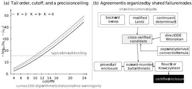

Panel (a) plots the reproduced Bessel data as $-\log_{10}|z_{N,K}-j_{0,1}|$. All three curves used 100-digit arithmetic; the binary64 line is a warning about the plateau that ordinary double precision would impose, not a clipping of the plotted data. Panel (b) groups algebraically related recurrence evaluators and separates them from an ODE Wronskian or a separately derived exact connection formula. Cross-agreement yields a candidate; a proved tail enclosure, outward-rounded arithmetic, and a Rouché or Krawczyk test yield a certificate.

The table makes two effects visible. At fixed $N$, a better tail seed gains several digits. At fixed tail order, increasing $N$ drives the error far below binary64 resolution. A double-precision computation would flatten while the mathematical approximation continued to improve.

A rigorous tail is a set, not a longer decimal

For the general three-term recurrence, write the backward Riccati map as

$$R_n = \Phi_n(R_{n+1}), \qquad \Phi_n(z) = - \frac{ \gamma_n }{ \beta_n+\alpha_nz }.$$

Suppose a theorem—not merely a formal asymptotic expansion—gives

$$\left| R_{N+1} - \widetilde R_{N+1} \right| \leq E_{N+1}.$$

Let $X_{n+1}$ contain both exact and approximate tails and define

$$d_n = \inf_{z\in X_{n+1}} \left| \beta_n+\alpha_nz \right|.$$

If $d_n>0$, then

$$\sup_{z\in X_{n+1}} \left| \Phi_n'(z) \right| \leq q_n, \qquad q_n = \frac{ |\alpha_n\gamma_n| }{ d_n^2 }.$$

Repeated use of the mean-value bound along a convex enclosure gives

$$\left| R_k-\widetilde R_k \right| \leq E_{N+1} \prod_{j=k}^{N}q_j.$$

If the endpoint residual is

$$F_0=\beta_0+\alpha_0R_1,$$

then

$$\left| F_0-\widetilde F_0 \right| \leq |\alpha_0| E_{N+1} \prod_{j=1}^{N}q_j.$$

Complex ball arithmetic can propagate the whole set $X_n=\Phi_n(X_{n+1})$ with outward rounding, often more sharply than the scalar product bound. Both routes require a proved starting enclosure. A formal $K$-term seed without a remainder theorem is still only an accelerated approximation.

If the ball

$$\beta_n+\alpha_nX_{n+1}$$

contains zero, the affine ratio chart has failed. Subdivide the parameter region or propagate homogeneous pairs projectively; do not divide through the ball. In an equal-root or nearly parabolic recurrence, $q_n$ may approach one. The resulting weak bound is an honest diagnosis of slow minimal–dominant separation.

Root finding is local; root counting is global

Newton’s method follows one local branch. It does not prove that all roots were found, that no root was counted twice, or that a nearby pole was not mistaken for a zero. For a meromorphic characteristic function,

$$\nu_\Gamma = \frac1{2\pi\ii} \oint_\Gamma \frac{ F'(\lambda) }{ F(\lambda) } \,\dd\lambda = N_Z-N_P.$$

The contour and its interior must lie in a domain of one declared analytic sheet on which $F$ is meromorphic. The contour must avoid every zero and pole and have a fixed positive orientation. For a ratio residual, certify the number of chart poles separately and recover the zero count from

$$N_Z=\nu_\Gamma+N_P.$$

An analytic homogeneous Wronskian, Casoratian, or determinant is usually safer.

For an analytic matrix function $T$ invertible on $\Gamma$,

$$\nu_\Gamma = \frac1{2\pi\ii} \oint_\Gamma \operatorname{tr} \left( T^{-1}T' \right) \,\dd\lambda$$

counts eigenvalues inside with algebraic multiplicity.

A numerically computed winding number close to an integer is evidence, not yet a certificate. Rigorous counting also needs validated quadrature or an enclosure that keeps the entire contour image away from zero. Finite sampling without an inter-sample derivative bound can miss a rapid winding.

Rouché converts enclosures into root counts

A compact local certificate is especially useful. Let $F$ be holomorphic on a neighborhood of the closed disk

$$\overline B(c,r).$$

Suppose outward-rounded computation proves

$$|F(c)|\leq\eta,$$

and, for some nonzero constant $a$,

$$\sup_{z\in\overline B(c,r)} \left| F'(z)-a \right| \leq M.$$

If

$$\eta+Mr < |a|r,$$

then $F$ has exactly one zero, counted with multiplicity, in $B(c,r)$.

Indeed, on $|z-c|=r$,

$$\begin{aligned} \left| F(z)-a(z-c) \right| &= \left| F(c) + \int_c^z \bigl(F'(\zeta)-a\bigr) \,\dd\zeta \right| \\ &\leq \eta+Mr < |a(z-c)|. \end{aligned}$$

Rouché’s theorem compares $F$ with the linear function $a(z-c)$, which has one zero in the disk.

For an infinite recurrence, the enclosures of $F(c)$ and $F'$ must include tail and evaluation errors; the computed center residual contributes to $\eta$. A certificate for $F_N$ alone is only a certificate for the finite approximant. A global finite-to-infinite bridge is

$$\sup_{\lambda\in\Gamma} \left| F(\lambda)-F_N(\lambda) \right| < \inf_{\lambda\in\Gamma} \left| F_N(\lambda) \right|.$$

When both functions are holomorphic on and inside $\Gamma$, this inequality proves that $F$ and $F_N$ have the same number of zeros there.

Krawczyk inclusion handles complex boxes

For a complex scalar equation, identify

$$\mathcal F(x,y) = \begin{pmatrix} \operatorname{Re}F(x+\ii y) \\ \operatorname{Im}F(x+\ii y) \end{pmatrix}$$

as a $C^1$ map $\mathbb R^2\to\mathbb R^2$ on a neighborhood of the real interval box $X$. Let $x_0\in X$, let $J(X)$ enclose every Jacobian on $X$, and let $C$ be a nonsingular point approximation to $J(x_0)^{-1}$. The Krawczyk operator is

$$\begin{aligned} K(x_0,X) ={}& x_0 - C\mathcal F(x_0) \\ &+ \left( I-CJ(X) \right) \left( X-x_0 \right). \end{aligned}$$

The strict inclusion

$$K(x_0,X) \subset \operatorname{int}X$$

proves that $X$ contains a unique zero. For holomorphic $F$,

$$J = \begin{pmatrix} \operatorname{Re}F' & -\operatorname{Im}F' \\ \operatorname{Im}F' & \operatorname{Re}F' \end{pmatrix}.$$

The real two-dimensional formulation avoids an invalid appeal to a complex mean-value theorem. Multiple roots require deflation, multiplicity-aware inclusion, or a root count rather than ordinary interval Newton.

An exact 10⁻⁴⁹ Bessel bracket

Observed convergence can now be upgraded. Define the exact rational endpoints

$$\begin{aligned} L &= 2.4048255576957727686216318793264546431242449091459, \\ U &= 2.4048255576957727686216318793264546431242449091460. \end{aligned}$$

Their separation is exactly $10^{-49}$. For rational $x$, every term in

$$J_0(x) = \sum_{k=0}^{\infty} (-1)^k \frac{ (x^2/4)^k }{ (k!)^2 }$$

is rational. Let $S_{50}(x)$ be the partial sum through $k=50$ and let $a_{51}(x)$ be the magnitude of the next term. From $k=1$ onward the term magnitudes decrease throughout $[L,U]$, so the alternating-series theorem gives

$$S_{50}(x)-a_{51}(x) < J_0(x) < S_{50}(x).$$

Exact integer arithmetic gives, at both endpoints,

$$a_{51}<6.1\times10^{-125},$$

and the outward rational sign bounds

$$\begin{aligned} 3.48533\times10^{-50} &< J_0(L) < 3.48534\times10^{-50}, \\ -1.70615\times10^{-50} &< J_0(U) < -1.70614\times10^{-50}. \end{aligned}$$

Existence follows from continuity. To prove uniqueness and identify the first positive zero, note first that $J_0(x)>0$ on $0\leq x\leq2$ by grouping its alternating series after $1-x^2/4$. Next,

$$J_1(2) > \sum_{k=0}^{5} \frac{ (-1)^k }{ k!(k+1)! } = \frac{49829}{86400} > 0.5767.$$

Bessel’s integral gives $|J_n(x)|\leq1$ for real $x$ and integer $n$. Together with

$$J_1' = \frac{ J_0-J_2 }{ 2 },$$

this implies $|J_1'|\leq1$. Hence, for $2\leq x\leq U$,

$$J_1(x) > 0.5767-0.405 > 0.$$

Since $J_0'=-J_1$, the function $J_0$ is strictly decreasing on $[2,U]$. The sign change therefore encloses exactly one zero, and positivity on $[0,2]$ makes it the first positive zero:

$$j_{0,1}\in[L,U].$$

This is a certificate, not a stability observation. It uses exact rational partial sums and analytic inequalities. Outward-rounded ball libraries such as Arb automate the same logic for functions whose terms are not rational.

As genuinely different numerical checks, one may evaluate

$$J_0(x) = \frac1\pi \int_0^\pi \cos(x\sin\theta) \,\dd\theta$$

or shoot the Bessel ODE from its regular Taylor series at the origin. Ordinary high-precision quadrature and ODE integration reproduce the bracket, but they remain cross-checks until their own truncation and integration errors are enclosed.

Independence is measured by shared failure modes

Two formulas can look different while representing the same finite algebra. The finite continuant determinant and its zero-tail continued fraction have the same zeros after cross-multiplication; agreement between them is useful for indexing, but not independent spectral evidence.

Comparison	Likely failures exposed	Evidence level
Larger $N$, $K$, and $p$	Tail, rounding, and asymptotic saturation	Internal refinement
Several split indices or match points	Ratio-chart and propagation failures	Internal refinement
Backward homogeneous sweep versus modified Lentz	Arithmetic and rescaling bugs	Independent evaluator, same representation
Continued fraction versus continuant determinant	Indexing and denominator poles	Algebraic cross-check, same finite object
Recurrence versus direct ODE Wronskian	Recurrence derivation, transfer, and endpoint errors	Strong representation independence
Separately derived exact connection formula or separate master equation	Model-specific derivation errors	Stronger representation independence
Tail balls plus Rouché or Krawczyk inclusion	Rounding, tail, existence, and uniqueness	Rigorous certification of the declared model

A second program that copies the same coefficient table still shares the same derivation error. Independence should be designed around failure modes, not programming languages or author names.

A research-grade QNM record

The Bessel problem is deliberately benign. A QNM computation adds branch cuts, exponentially growing endpoint representatives, nonnormality, and often a coupled angular eigenvalue. The following workflow upgrades the chapter’s recurrence calculation without overclaiming.

1. Freeze the Fourier convention, units, spectral coordinate, endpoint gauges, branch cuts, uniformizer, analytic sheet, exceptional recurrence rows, and physical boundary conditions.

2. Evaluate the minimal tail backward with homogeneous pairs or a safe ratio chart. Derive a $K$-term large-order seed and differentiate the seed when computing $F'$.

3. Refine $N$, $K$, $p$, split index, and root-solver tolerance separately. Track zeros and nearby ratio poles together.

4. Count roots on a contour before polishing them locally. Continue a simple branch with

   $$\frac{\dd\lambda}{\dd\mu} = - \frac{ F_\mu }{ F_\lambda },$$

   and switch to pseudo-arclength continuation when $F_\lambda$ becomes small.

5. Build a separately derived ODE calculation: endpoint-adapted expansions, stable-direction integration, Abel-normalized Wronskians at several match points, and variational equations for spectral derivatives.

6. For damped outgoing waves, test an admissible complex contour, exterior complex scaling, or a hyperboloidal formulation rather than trusting an exponentially ill-conditioned real-axis shooting path.

7. If the angular and radial equations are coupled, solve the two conditions simultaneously with the full Jacobian. Nearest-frequency sorting is not a branch-tracking method near collisions.

As a recurrence control, use the four-correction Schwarzschild tail derived on the large-order asymptotics page. The target is the positive-real fundamental gravitational mode—modern overtone index $n=0$, the first QNM in Leaver’s original numbering. Using 80 decimal digits and tolerance $10^{-68}$, a secant solve started from

$$\omega^{(0)}=0.75-0.18\,\ii$$

under the conventions

$$\ee^{-\ii\omega t}, \qquad 2M=1, \qquad s=2, \qquad \ell=2.$$

The values below use the same recurrence at several depths; the last column is only a difference from the $N=400$ value, not an error bound.

| $N$ | $\omega_N$ | $|\omega_N-\omega_{400}|$ | |---:|---|---:| | 50 | $0.747343368836111112-0.177924631377816164\,\ii$ | $6.17\times10^{-14}$ | | 100 | $0.747343368836083673-0.177924631377871397\,\ii$ | $1.54\times10^{-18}$ | | 200 | $0.747343368836083672-0.177924631377871397\,\ii$ | $9.78\times10^{-25}$ | | 400 | $0.747343368836083672-0.177924631377871397\,\ii$ | reference row |

The $N=200$ and $N=400$ rows agree to the displayed precision; the earlier rows show the approach to that plateau. At $N=200$, tail orders $K=0,\ldots,4$ differed from a depth-$3200$, $K=4$ reference by between $9.78\times10^{-25}$ and $4.45\times10^{-20}$. Working-precision sweeps from $30$ through $80$ decimal digits preserved the displayed digits. These are still observed differences, not error bounds.

The evidence therefore supports a cutoff-, tail-order-, and precision-stable recurrence candidate. It does not include a split-chart audit, a rigorous asymptotic remainder, or a separately implemented ODE Wronskian. Calling it internally converged under the strict definition at the start of this page, independently cross-verified, or certified would be unjustified.

Reproduction manifest

Every publishable root should carry a compact record.

Field	What to record
Mathematical object	Differential equation or pencil, recurrence, row normalization, and transfer map
Physical conventions	Units, Fourier sign, endpoint meaning, source/response normalization
Analytic conventions	Branches, cuts, sheet, uniformizer, and continuation path
Discretization	Cutoff $N$, tail order $K$, explicit seed, basis size, and omitted-row residual
Arithmetic	Precision in bits or decimal digits, rounding mode, coefficient provenance
Local solve	Initial guess, solver, tolerance, analytic derivative, residual, Newton correction
Conditioning	Declared residual scale, backward error, left–right or Wronskian condition estimate
Global audit	Contour, winding or zero–pole count, distance of the contour image from zero
Independence	Separate representation, its own refinements, and final disagreement
Claim	Reported digits and one of computed, internally converged, cross-verified, or certified
Reproduction	Script revision, software versions, raw refinement table, and deterministic inputs

For the two control experiments on this page, the linked script records the decimal-string inputs, coefficient formulas, terminal seeds, solver starts and tolerances, cutoffs, precision sweeps, software versions, and raw tables. Its exact-rational Bessel branch is a certificate; its mpmath recurrence branches are convergence audits.

Later conformal-block, isomonodromic, exact-WKB, gauge-theory, ODE/IM, and TBA formulas should reproduce this direct-method record wherever a complete dictionary exists. Agreement is most informative when each method keeps its own normalization and branch ledger until the final comparison.

Common pitfalls

Stable digits without a bound. Several truncations may approach the same biased limit. Report the observed grid and reserve certified digits for an enclosure theorem.

A small residual without conditioning. Residual is backward error only after a scale is declared, and nonnormality can magnify it enormously. Report a left–right, Wronskian, or structured condition estimate.

Fixed-precision over-refinement. Increasing cutoff after arithmetic has saturated can produce a plateau or an upturn. Vary cutoff and precision on separate axes.

Promoted low-precision inputs. A binary64 coefficient stored in a 200-digit container still carries about sixteen decimal digits. Parse exact or high-precision data at their source precision.

A frozen asymptotic derivative. Differentiating a recurrence while holding its parameter-dependent tail seed fixed gives the wrong $F'$. Differentiate the seed and propagate its derivative.

A finite certificate advertised as infinite. A ball for $F_N$ proves a statement about $F_N$. Enclose $F-F_N$ on the relevant disk or contour before transferring the count.

A sampled contour advertised as a root count. Phase can wind between samples. Bound derivatives or use validated quadrature and prove that the whole contour image avoids zero.

A meromorphic ratio treated as analytic. The argument principle returns $N_Z-N_P$. Prefer a homogeneous analytic determinant or keep a pole ledger.

Nearest-neighbor mode tracking. Roots exchange, collide, or circle branch points. Use predictors, eigenvector overlap, pseudo-arclength continuation, and cluster root counts.

Algebraic identity mistaken for independence. A finite determinant and its continued fraction may be the same continuant. Compare failure modes, not surface syntax.

Exercises

1. Complete the recurrence residual

Let $T_Nu=0$ be the first $N+1$ rows of a three-term recurrence and extend $u_0,\ldots,u_N$ by zeros. Show that the infinite residual need not vanish. Which additional row appears, and what does a self-adjoint residual bound imply?

Solution

Rows $0,\ldots,N$ vanish by assumption. The extended sequence has $u_{N+1}=u_{N+2}=\cdots=0$. At row $N+1$,

$$\begin{aligned} (Tu)_{N+1} &= \alpha_{N+1}u_{N+2} + \beta_{N+1}u_{N+1} + \gamma_{N+1}u_N \\ &= \gamma_{N+1}u_N. \end{aligned}$$

Later rows vanish. Thus the full residual norm contains at least $|\gamma_{N+1}u_N|$ in the unweighted $\ell^2$ norm. A finite eigenvector whose last component is not small can therefore be a poor approximate infinite eigenvector even when every retained equation is solved exactly.

If $T=A-\widehat\lambda I$ with $A$ self-adjoint and $\|u\|=1$, the spectral theorem gives

$$\operatorname{dist} \bigl( \widehat\lambda,\sigma(A) \bigr) \leq \|Tu\|.$$

This encloses some spectral point. A gap, index theorem, or Sturm count is still required to identify it. No analogous normal-distance conclusion holds for a general nonnormal operator.

2. Prove the Wronskian perturbation bound

For $F=\det(x,y)$, prove

$$|\delta F| \leq \left( \varepsilon_x+\varepsilon_y+\varepsilon_x\varepsilon_y \right) \|x\|_2\|y\|_2$$

under the relative jet bounds used above. Show that $\|x\|\|y\|/|F'|$ is invariant at a root under separate analytic rescalings of the jets.

Solution

Bilinearity gives

$$\begin{aligned} \delta F ={}& \det(x+\delta x,y+\delta y) - \det(x,y) \\ ={}& \det(\delta x,y) + \det(x,\delta y) + \det(\delta x,\delta y). \end{aligned}$$

For two vectors in $\mathbb C^2$,

$$|\det(a,b)| \leq \|a\|_2\|b\|_2.$$

Applying this inequality to the three terms and substituting the relative bounds proves the claim.

Now replace

$$x\mapsto a(\lambda)x, \qquad y\mapsto b(\lambda)y,$$

where $a$ and $b$ are analytic and nonzero near $\lambda_*$. Then

$$\widetilde F=abF.$$

At a root $F(\lambda_*)=0$,

$$\widetilde F'(\lambda_*) = a(\lambda_*)b(\lambda_*)F'(\lambda_*).$$

The product of jet norms is also multiplied by $|a(\lambda_*)b(\lambda_*)|$. Their ratio is unchanged. The result does not remove dependence on the spectral coordinate, ODE gauge, or chosen jet norm.

3. Audit the nonnormal two-by-two example

For $A_\varepsilon$ above:

1. derive the eigenvalues and left and right eigenvectors;
2. compute their condition numbers;
3. exhibit a perturbation of norm $\varepsilon^2$ that makes $\widehat\lambda=1$ exact;
4. prove by Rouché that each disk $|\lambda-\lambda_\pm|<\varepsilon/2$ contains exactly one eigenvalue.

Solution

The characteristic determinant is

$$D_\varepsilon(\lambda) = \det(A_\varepsilon-\lambda I) = (\lambda-1)^2-\varepsilon^2.$$

Thus $\lambda_\pm=1\pm\varepsilon$. Direct substitution gives the stated $v_\pm$ and $w_\pm$. Since $T'=-I$,

$$\left| w_\pm^*T'v_\pm \right| = 2\varepsilon,$$

while

$$\|v_\pm\|_2\|w_\pm\|_2 = 1+\varepsilon^2.$$

Hence

$$\kappa_{\mathrm{abs}} = \frac{1+\varepsilon^2}{2\varepsilon}.$$

At $\lambda=1$ the residual for $e_1$ is $\varepsilon^2e_2$. The rank-one perturbation

$$\Delta A = - \varepsilon^2e_2e_1^*$$

has spectral norm $\varepsilon^2$ and satisfies

$$\left( A_\varepsilon+\Delta A-I \right)e_1=0.$$

Finally, near $\lambda_+=1+\varepsilon$, put $w=\lambda-\lambda_+$. Then

$$D_\varepsilon(\lambda) = 2\varepsilon w+w^2.$$

On $|w|=\varepsilon/2$,

$$|w^2| = \frac{\varepsilon^2}{4} < \varepsilon^2 = |2\varepsilon w|.$$

Rouché compares $D_\varepsilon$ with $2\varepsilon w$, proving one zero in the disk. The calculation around $\lambda_-$ is identical after changing the sign of the linear term.

4. Propagate a terminal tail error

Prove the product bound

$$\left| R_k-\widetilde R_k \right| \leq E_{N+1} \prod_{j=k}^{N}q_j$$

for the backward Möbius maps. Explain what fails when a denominator enclosure contains zero.

Solution

Assume both arguments remain in the convex set $X_{n+1}$. Along the line segment joining them,

$$\begin{aligned} \left| \Phi_n(R_{n+1}) - \Phi_n(\widetilde R_{n+1}) \right| &\leq \sup_{z\in X_{n+1}} |\Phi_n'(z)| \left| R_{n+1}-\widetilde R_{n+1} \right| \\ &\leq q_n \left| R_{n+1}-\widetilde R_{n+1} \right|. \end{aligned}$$

Iterating from the terminal estimate gives the product.

The derivative is

$$\Phi_n'(z) = \frac{ \alpha_n\gamma_n }{ (\beta_n+\alpha_nz)^2 },$$

so $d_n>0$ yields the stated $q_n$. If the denominator set contains zero, the affine map is unbounded and no finite Lipschitz constant follows. This may be a chart pole rather than a singular solution. Propagate homogeneous pairs, use a reciprocal chart, or subdivide the parameter box instead of dividing by an interval that contains zero.

5. Prove the local Rouché certificate

Starting from the bounds

$$|F(c)|\leq\eta, \qquad \sup_{\overline B(c,r)} |F'-a| \leq M,$$

prove that $\eta+Mr<|a|r$ implies exactly one zero in the disk. Why does the same calculation not certify an infinite recurrence when it is applied only to $F_N$?

Solution

For $|z-c|=r$, integrate along the straight segment inside the disk:

$$F(z) - a(z-c) = F(c) + \int_c^z \bigl(F'(\zeta)-a\bigr) \,\dd\zeta.$$

Therefore

$$\left| F(z)-a(z-c) \right| \leq \eta+Mr < |a|r = |a(z-c)|.$$

Rouché’s theorem gives the same zero count as $a(z-c)$, namely one.

Applying this proof to $F_N$ establishes a theorem about $F_N$. To transfer it to the exact function, one must also enclose $F-F_N$ on the boundary and keep the total perturbation strictly below the comparison function. That extra estimate is precisely the infinite-tail problem.

6. Reproduce the rational Bessel certificate

Verify the alternating bounds at $L$ and $U$, and prove that the enclosed zero is $j_{0,1}$. Which parts are exact, and which alternative computations would merely cross-verify the result?

Solution

Treat $L$ and $U$ as integers divided by $10^{49}$. Every term of the $J_0$ series is then rational. For

$$a_k = \frac{(x^2/4)^k}{(k!)^2},$$

the ratio is

$$\frac{a_{k+1}}{a_k} = \frac{x^2/4}{(k+1)^2}.$$

On $[L,U]$ this is less than one for every $k\geq1$. Since $50$ is even, the next term is negative and

$$S_{50}-a_{51} < J_0 < S_{50}.$$

Exact fraction comparison gives the two sign intervals printed in the main text and $a_{51}<6.1\times10^{-125}$.

For $0\leq x\leq2$, put $t=x^2/4\leq1$. The alternating tail after $1-t$ begins with a positive decreasing term, so $J_0(x)>0$. At $x=2$, the $J_1$ series has a negative-ending lower partial sum

$$\sum_{k=0}^{5} \frac{(-1)^k}{k!(k+1)!} = \frac{49829}{86400} > 0.5767.$$

The integral bound $|J_n|\leq1$ and the derivative recurrence imply $|J_1'|\leq1$. Thus $J_1>0$ on $[2,U]$, so $J_0'=-J_1<0$ there. The sign change between $L$ and $U$ is unique and no earlier positive zero exists.

The rational sums and comparisons are exact; the analytic alternating, integral, and derivative bounds complete the proof. A high-precision continued fraction, numerical integral, or ODE shooting computation is a valuable independent check but is not a certificate unless its own errors are outward-rounded and bounded.

7. Classify a verification suite

A QNM code performs the following tests:

• doubles the continued-fraction depth;
• evaluates the same fraction with modified Lentz;
• compares against a continuant determinant built from the same coefficients;
• varies an ODE match point;
• compares the recurrence root with a separately derived ODE Wronskian;
• encloses the recurrence tail and applies Krawczyk inclusion.

Classify the evidence supplied by each test and identify one model error that all recurrence-only checks could share.

Solution

Doubling depth is an internal tail-refinement test. Modified Lentz supplies an independent arithmetic evaluator but uses the same analytic continued fraction. The continuant determinant is an algebraic cross-check of the same finite recurrence and is especially useful for detecting index shifts and ratio poles. Varying an ODE match point is an internal propagation test for the ODE representation.

The separately derived ODE Wronskian supplies strong representation independence: it can detect a bad recurrence derivation, a faulty recurrence-to-ODE transfer, or a wrong minimal-tail interpretation. The tail enclosure plus Krawczyk inclusion supplies certification if the arithmetic, derivative, and infinite-tail bounds all satisfy the theorem’s hypotheses.

Every recurrence-only test could share a sign error in a recurrence coefficient, a wrong spin or angular-separation convention, or an incorrect translation from minimal sequence behavior to the physical endpoint condition. Those are model or dictionary errors, not floating-point errors.

References

• NIST Digital Library of Mathematical Functions, §3.6, “Linear Difference Equations”, for recurrence stability and backward algorithms, and §3.10, “Continued Fractions”, for numerical evaluation.
• NIST Digital Library of Mathematical Functions, §10.2, “Definitions”, §10.6, “Recurrence Relations and Derivatives”, §10.9, “Integral Representations”, and §10.21, “Zeros”, for the certified Bessel benchmark.
• W. Gautschi, “Computational Aspects of Three-Term Recurrence Relations”, SIAM Review 9 (1967), 24–82, for minimal solutions, Miller recursion, continued fractions, and error analysis.
• F. W. J. Olver, “Numerical Solution of Second-Order Linear Difference Equations”, Journal of Research of the National Bureau of Standards B 71B (1967), 111–129, for stable boundary-value algorithms for recurrences.
• N. J. Higham, Accuracy and Stability of Numerical Algorithms, 2nd ed., SIAM, 2002, for floating-point models, backward error, conditioning, and precision budgeting.
• S. Güttel and F. Tisseur, “The Nonlinear Eigenvalue Problem”, Acta Numerica 26 (2017), 1–94, for weighted backward errors, left–right condition numbers, pseudospectra, and contour counts.
• L. N. Trefethen and M. Embree, Spectra and Pseudospectra, Princeton University Press, 2005, for nonnormal residual sensitivity.
• L. M. Delves and J. N. Lyness, “A Numerical Method for Locating the Zeros of an Analytic Function”, Mathematics of Computation 21 (1967), 543–560, for argument-principle root location.
• S. M. Rump, “Verification Methods: Rigorous Results Using Floating-Point Arithmetic”, Acta Numerica 19 (2010), 287–449, for interval and floating-point verification methods.
• R. E. Moore, R. B. Kearfott, and M. J. Cloud, Introduction to Interval Analysis, SIAM, 2009, especially Chapter 8 for interval Newton and Krawczyk inclusion.
• F. Johansson, “Arb: Efficient Arbitrary-Precision Midpoint-Radius Interval Arithmetic”, IEEE Transactions on Computers 66 (2017), 1281–1292, for arbitrary-precision ball arithmetic and rigorous special-function evaluation.
• H.-P. Nollert, “Quasinormal Modes of Schwarzschild Black Holes: The Determination of Quasinormal Frequencies with Very Large Imaginary Parts”, Physical Review D 47 (1993), 5253–5258, for accelerated continued-fraction tails in QNM computations.
• E. W. Leaver, “An Analytic Representation for the Quasi-Normal Modes of Kerr Black Holes”, Proceedings of the Royal Society A 402 (1985), 285–298, for the recurrence coefficients, mode convention, continued-fraction condition, and original Schwarzschild frequency table.
• G. B. Cook and M. Zalutskiy, “Gravitational Perturbations of the Kerr Geometry: High-Accuracy Study”, Physical Review D 90 (2014), 124021, for high-accuracy Kerr mode calculations coupling a spectral angular method to a radial continued-fraction method.

Part I control group complete

The four chapters of Part I now supply the local ODE, global analytic, special-function, Wronskian, recurrence, Green-function, and verification control group for the book. Part II begins by replacing fixed singularities with isomonodromic motion while preserving the monodromy data.