Inverse Monodromy and Conditional Spectral Constraints

A spectrum begins with a boundary intersection, not with a tau function. For a second-order ODE, two endpoint or sectorial conditions select two one-dimensional solution spaces. Their Wronskian vanishes exactly when the spaces coincide. Monodromy can encode that coincidence, and an isomonodromic tau function can sometimes solve the resulting inverse problem, but each translation adds hypotheses.

The distinction is decisive in Heun and black-hole applications. A raw Jimbo–Miwa–Ueno (JMU) tau zero records failure of a normalized inverse Riemann–Hilbert problem. A neighboring tau zero can instead encode the collision that removes an apparent scalar singularity. Neither event is a quantization condition or quasinormal mode (QNM) condition until the physical boundary lines, analytic sheet, spectral-parameter dictionary, and accessory constraint have also been imposed.

First pass

Follow the upper route in the figure below: boundary lines → Wronskian → spectral zero. Then read the lower inverse-monodromy route as a representation of the same condition that must be proved equivalent, not as a replacement for the boundary problem.

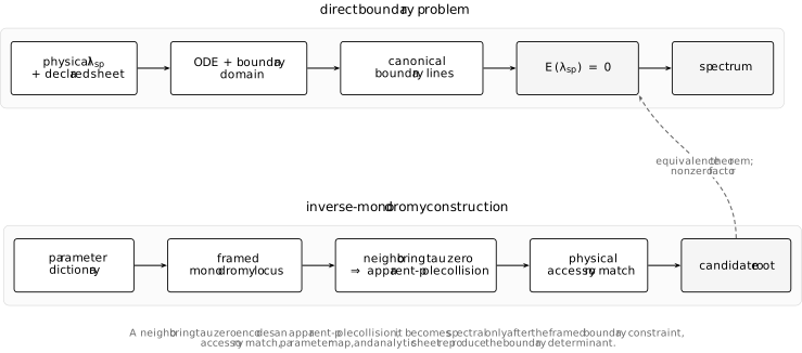
The upper lane gives the direct spectral-zero condition. The lower lane represents that zero through monodromy and isomonodromy only after the parameter dictionary, boundary flags, neighboring-tau specialization, independent accessory match, and analytic sheet have been fixed. A dashed bridge is an equivalence theorem to prove, not an automatic identity.

The boundary Wronskian is the primary zero

Let $\lambda_{\mathrm{sp}}$ vary in a parameter domain $\Omega$ on which the ODE

$$y'' + p(z,\lambda_{\mathrm{sp}})y' + q(z,\lambda_{\mathrm{sp}})y =0$$

has two analytically chosen boundary solutions:

• $y_L^+(z,\lambda_{\mathrm{sp}})$ satisfies the declared left endpoint, horizon, or sectorial condition;
• $y_R^+(z,\lambda_{\mathrm{sp}})$ satisfies the declared right endpoint, infinity, or sectorial condition.

The superscript $+$ is a label for the selected line, not a claim about a sign of energy or frequency. Fix the continuation paths, branches, and analytic sheet before comparing the two solutions. The Abel-normalized boundary function is

$$\begin{aligned} E(\lambda_{\mathrm{sp}}) = \exp\left( \int_{z_*}^{z} p(s,\lambda_{\mathrm{sp}})\,\dd s \right) \Wr[y_L^+,y_R^+](z,\lambda_{\mathrm{sp}}). \end{aligned}$$

Abel’s identity makes $E$ independent of the matching point. In Liouville normal form, $p=0$ and the ordinary Wronskian is already constant. On a domain where both boundary lines are analytic and nonzero,

$$E(\lambda_{\mathrm{sp},*})=0 \quad\Longleftrightarrow\quad \mathbb C y_L^+(\lambda_{\mathrm{sp},*}) = \mathbb C y_R^+(\lambda_{\mathrm{sp},*}).$$

This is the homogeneous boundary condition. Whether its zero is an eigenvalue, a resonance, or a QNM depends on the operator domain and sheet declared on the spectral-theory page.

One connection entry carries the condition

Complete the selected solutions to canonical local frames

$$\Phi_L=(y_L^+,y_L^-), \qquad \Phi_R=(y_R^+,y_R^-),$$

and use the book convention

$$\Phi_R=\Phi_LC_{LR}, \qquad C_{LR} = \begin{pmatrix} c_{11}&c_{12}\\ c_{21}&c_{22} \end{pmatrix}.$$

The first column says

$$y_R^+ = c_{11}y_L^+ + c_{21}y_L^-.$$

Consequently,

$$\Wr[y_L^+,y_R^+] = c_{21}\Wr[y_L^+,y_L^-],$$

and hence, for a nondegenerate left frame,

$$E(\lambda_{\mathrm{sp}})=0 \quad\Longleftrightarrow\quad c_{21}(\lambda_{\mathrm{sp}})=0.$$

Changing a selected solution or a complementary basis vector by a nowhere-zero analytic factor changes $E$ and $c_{21}$ by possibly different nowhere-zero factors; a left selected-line rescaling, for example, cancels from the Wronskian ratio defining $c_{21}$. Their zero divisors are nevertheless unchanged. A rescaling that vanishes, blows up, or changes branch at $\lambda_{\mathrm{sp},*}$ is not an admissible normalization change for this conclusion.

Boundary lines define a framed monodromy locus

Assume first that both endpoints are nonresonant regular singularities. The scalar equation need not initially have determinant-one monodromy. Before using trace coordinates, choose a coherent square-root lift of its determinant character and set

$$\widehat M_j = (\det M_j)^{-1/2}M_j \in SL(2,\mathbb C).$$

Equivalently, pass to the Liouville or traceless-system gauge. This central normalization preserves every local eigenline; it only fixes the scalar factors needed by the Fricke formulas. In what follows, suppress the hats and let $\theta_j$ denote the lifted exponent difference. In the corresponding eigenbases,

$$D_j = \begin{pmatrix} \ee^{\pi\ii\theta_j}&0\\ 0&\ee^{-\pi\ii\theta_j} \end{pmatrix}, \qquad j=L,R.$$

Use the $L$ frame as the based frame. Then

$$M_L=D_L, \qquad M_R=C_{LR}D_RC_{LR}^{-1}.$$

If $c_{21}=0$, the connection matrix is upper triangular. The selected first line is invariant under both $M_L$ and $M_R$, with eigenvalues $\ee^{\pi\ii\theta_L}$ and $\ee^{\pi\ii\theta_R}$. Thus the boundary condition implies

$$\operatorname{tr}(M_LM_R) = 2\cos\!\left[ \pi(\theta_L+\theta_R) \right].$$

For selected local signs $s_L,s_R\in\{+1,-1\}$, the corresponding formula is

$$p_{LR} := \operatorname{tr}(M_LM_R) = 2\cos\!\left[ \pi(s_L\theta_L+s_R\theta_R) \right].$$

This is the familiar composite-exponent constraint. It remembers an eigenvalue pairing only modulo the even shifts and sign ambiguity of the cosine. The actual boundary condition also remembers which framed local lines were selected.

The trace sees two boundary branches at once

The loss of the flag is visible in one exact calculation. Set

$$a=\ee^{\pi\ii\theta_L}, \qquad b=\ee^{\pi\ii\theta_R},$$

and retain a general, not necessarily determinant-one, connection matrix $C_{LR}=(c_{jk})$. Direct multiplication gives

$$\begin{aligned} &\operatorname{tr}(M_LM_R) - \left[ ab+(ab)^{-1} \right] \\ &\qquad = \frac{ (a-a^{-1})(b-b^{-1}) }{ \det C_{LR} } c_{12}c_{21}. \end{aligned}$$

The two off-diagonal entries have invariant Wronskian descriptions, with all Wronskians evaluated at one common matching point:

$$\begin{aligned} c_{21} &= \frac{ \Wr[y_L^+,y_R^+] }{ \Wr[y_L^+,y_L^-] }, \\ c_{12} &= - \frac{ \Wr[y_L^-,y_R^-] }{ \Wr[y_L^+,y_L^-] }, \\ \det C_{LR} &= \frac{ \Wr[y_R^+,y_R^-] }{ \Wr[y_L^+,y_L^-] }. \end{aligned}$$

Therefore

$$\begin{aligned} &\operatorname{tr}(M_LM_R) - \left[ ab+(ab)^{-1} \right] \\ &= - (a-a^{-1})(b-b^{-1}) \\ &\quad\times \frac{ \Wr[y_L^+,y_R^+]\, \Wr[y_L^-,y_R^-] }{ \Wr[y_L^+,y_L^-]\, \Wr[y_R^+,y_R^-] }. \end{aligned}$$

Provided the frames are nondegenerate and neither $a$ nor $b$ equals $\pm1$, the composite-trace equation detects the union

$$c_{21}=0 \qquad\text{or}\qquad c_{12}=0.$$

The first component is the declared boundary problem; the second aligns the complementary local lines. Within this diagonal calculation, the semisimple limit $a=\pm1$ makes $D_L=\pm I$—and similarly for $b$—so the trace difference vanishes for every $C_{LR}$ and loses even this union. A genuinely logarithmic resonant point is different: its monodromy can have a Jordan part, the assumed eigenbasis does not exist, and the displayed factorization does not apply. Such a problem must be reformulated with Levelt flags and its trace condition rederived.

Reducibility is coarser than the boundary condition

Set

$$\kappa_L=\operatorname{tr}M_L, \qquad \kappa_R=\operatorname{tr}M_R, \qquad p=p_{LR}.$$

Two $SL(2,\mathbb C)$ matrices have a common invariant line precisely when their character lies on the reducible locus

$$\mathcal R_{LR} := \kappa_L^2+\kappa_R^2+p^2 - \kappa_L\kappa_Rp - 4 =0.$$

Equivalently, $\operatorname{tr}[M_L,M_R]=2$. Substituting the displayed composite trace makes $\mathcal R_{LR}=0$, as it must.

Writing

$$\kappa_L=2\cos A, \qquad \kappa_R=2\cos B,$$

exhibits the two components explicitly:

$$\begin{aligned} \mathcal R_{LR} ={}& \left[ p-2\cos(A+B) \right] \\ &\times \left[ p-2\cos(A-B) \right]. \end{aligned}$$

The converse does not recover $c_{21}=0$ from the coarse character alone. It identifies a pair-reducibility divisor, not a component with an oriented flag. Nor does a common line for $M_L$ and $M_R$ make an entire four-puncture representation reducible: every remaining generator must preserve the same line. A physical boundary condition is therefore a locus in a framed or decorated monodromy space. The Fricke traces give a useful invariant check, but they forget the flag that distinguishes the desired connection entry.

At an irregular endpoint, replace local eigenlines by canonical sectorial lines. The relevant boundary equation may be the vanishing of a Stokes multiplier or of an entry in a link matrix between sectorial bases. Ordinary total-monodromy traces generally do not remember which ingoing, outgoing, dominant, or recessive sectorial solution was chosen.

Direct and inverse monodromy solve opposite problems

Fix the true singularity positions and local exponent lifts of a scalar four-point equation. Varying its accessory $q_{\mathrm H}$ gives a direct Riemann–Hilbert map

$$q_{\mathrm H} \longmapsto [\rho(q_{\mathrm H})] \in \mathcal M_{\mathrm B}.$$

The direct spectral problem starts from a physical parameter $\lambda_{\mathrm{sp}}$, computes

$$\bigl( t_{\mathrm{phys}}(\lambda_{\mathrm{sp}}), \boldsymbol\theta_{\mathrm{phys}}(\lambda_{\mathrm{sp}}), q_{\mathrm{phys}}(\lambda_{\mathrm{sp}}) \bigr),$$

and asks whether $[\rho(q_{\mathrm{phys}}(\lambda_{\mathrm{sp}}))]$ lies on the framed boundary locus $\mathcal B_{LR}$ defined by $c_{21}=0$.

The inverse monodromy problem reverses this order. It starts with a monodromy point $\mathcal M\in\mathcal B_{LR}$ and reconstructs a connection or scalar accessory having those global data. The answer can be multivalued, can change bundle charts, and can fail to be represented by a normalized trivial-bundle Riemann–Hilbert problem at a Malgrange divisor. Isomonodromic deformation is useful because it moves the singular positions while keeping $\mathcal M$ fixed, so Hamiltonians and tau functions can reconstruct the accessory along that leaf.

Three tau zeros answer three different questions

The phrase “set tau to zero” is incomplete until the tau function and its restricted parameter family have been named.

Zero being imposed	What it means before further input	What is still missing for a spectrum
$\tau(t;\mathcal M)=0$ for fixed generalized monodromy $\mathcal M$	The deformation point lies on the Malgrange divisor, where the normalized inverse Riemann–Hilbert problem fails	A boundary problem and a map from $\lambda_{\mathrm{sp}}$ to $(t,\mathcal M)$
$\tau_{\rho^+}(t_0)=0$ in the Schlesinger-neighbor relation of the Heun-reduction page	The apparent scalar point collides with the declared true pole, on the chosen branch	The boundary monodromy locus and the physical accessory equation
$\mathcal T_B(\lambda_{\mathrm{sp}})=0$ after restricting to boundary data	A spectral condition only if $\mathcal T_B$ is proved equivalent to the boundary function	A nonzero-factor theorem, sheet control, and operator or response interpretation

For the first row, the Malgrange–Miwa theorem gives

$$\operatorname{div}_0\tau(\,\cdot\,;\mathcal M) = \mathcal D_{\mathcal M}.$$

The monodromy data have not disappeared at $\mathcal D_{\mathcal M}$. The chosen normalized factorization or trivial-bundle chart fails. The geometric connection persists on the resulting bundle, while residue-coordinate representatives may continue meromorphically after a change of bundle or elementary-transformation chart.

For the second row, a Schlesinger identity gives the extra interpretation of the neighboring divisor as an apparent-pole collision. The base $\tau_{\mathrm J}(\rho;t)$ is generally nonzero there and supplies the accessory through its logarithmic derivative. The neighboring and base tau functions must not be interchanged.

The third row is the only one that can immediately share a spectral zero set, and only after $\mathcal T_B$ has been constructed on the boundary monodromy locus and compared with $E$.

The Heun–Painlevé constraint stack

Suppose a physical reduction produces a general Heun equation with

$$t=t_{\mathrm{phys}}(\lambda_{\mathrm{sp}}), \qquad \boldsymbol\vartheta = \boldsymbol\vartheta_{\mathrm{phys}}(\lambda_{\mathrm{sp}}), \qquad q_{\mathrm H} = q_{\mathrm{phys}}(\lambda_{\mathrm{sp}}).$$

Let $\rho$ denote the shifted Painlevé VI (PVI) monodromy data required by the scalar collision convention on the Heun-reduction page. The unknowns normally include $\lambda_{\mathrm{sp}}$ and one or more composite monodromy coordinates inside $\rho$. A convention-complete inverse problem has the schematic form

$$\begin{aligned} \boldsymbol\theta(\rho) &= \boldsymbol\theta_{\mathrm{shift}} \bigl( \boldsymbol\vartheta_{\mathrm{phys}}(\lambda_{\mathrm{sp}}) \bigr), \\ F_B(\rho;\lambda_{\mathrm{sp}}) &=0, \\ \tau_{\rho^+} \bigl( t_{\mathrm{phys}}(\lambda_{\mathrm{sp}}) \bigr) &=0, \\ q_{\mathrm{phys}}(\lambda_{\mathrm{sp}}) &= \mathcal Q_\tau \bigl( \rho;t_{\mathrm{phys}}(\lambda_{\mathrm{sp}}) \bigr). \end{aligned}$$

The base inverse problem must remain in its declared chart:

$$\tau_{\mathrm J} \bigl( \rho;t_{\mathrm{phys}}(\lambda_{\mathrm{sp}}) \bigr) \ne0.$$

The four lines have different jobs:

1. the first fixes the integer-shifted local exponent dictionary;
2. $F_B=0$ selects the framed boundary or wild-monodromy locus;
3. the neighboring tau zero removes the apparent scalar singularity;
4. the accessory equation matches the reconstructed Heun equation to the physical one.

In the convention fixed on the Heun-reduction page,

$$\begin{aligned} \mathcal Q_\tau(\rho;t) ={}& t\alpha_{\mathrm H}\beta_{\mathrm H} \\ &+ t(t-1) \left[ \frac{\partial}{\partial t} \log\tau_{\mathrm J}(\rho;t) - \frac{\theta_0\theta_t}{2t} - \frac{\theta_1\theta_t}{2(t-1)} \right]. \end{aligned}$$

The formula assumes that the base tau is nonzero and that the collision is on the finite shifted-momentum branch used there. Other cyclic vectors, integer lifts, and collision poles change the printed equations.

Solving only $\tau_{\rho^+}(t_{\mathrm{phys}}(\lambda_{\mathrm{sp}}))=0$ produces an isomonodromic specialization, not a spectrum. Solving only $F_B=0$ produces a monodromy boundary locus, not necessarily the physical accessory. Generically the complete system is discrete only when all unknown monodromy coordinates and all independent equations have been counted and a transversality condition holds.

Modified Mathieu: collision plus normalizability

The modified Mathieu operator supplies an exact tau-function benchmark in which the logical separation can be read directly from the equations. For $t>0$, consider

$$\left[ - \frac{\dd^2}{\dd x^2} + 2\sqrt t\cosh x \right]\Psi = E\Psi, \qquad \Psi\in L^2(\mathbb R).$$

In the Painlevé III(D₈) construction of Bershtein, Gavrylenko, and Grassi, the two monodromy coordinates are $(\sigma,\eta)$. Removing the auxiliary scalar singularity on the $w=\infty$ branch gives

$$\mathcal T_1(\sigma,\eta,t)=0.$$

This is their singularity-matching condition, not yet the $L^2(\mathbb R)$ condition. The connection matrix between the canonical bases at the two irregular ends is, away from $\sin(2\pi\sigma)=0$,

$$\mathsf C = \frac{1}{\sin(2\pi\sigma)} \begin{pmatrix} \sin(\eta/2) & -\ii\sin(2\pi\sigma+\eta/2) \\ \ii\sin(2\pi\sigma-\eta/2) & \sin(\eta/2) \end{pmatrix}.$$

Mapping the decaying line at one end to the decaying line at the other requires the appropriate diagonal connection entries to vanish:

$$\sin\frac{\eta}{2}=0.$$

Only the intersection of the collision divisor with this boundary locus is spectral. On the branch $\eta=0$, the Bäcklund relation

$$\mathcal T_1(\sigma,\eta,t) \sim \mathcal T_0 \left( \sigma+\frac12,\eta,t \right)$$

uses the canonical normalization of that construction. Here $\sim$ means proportionality by a factor that is nonzero on the chosen monodromy chart; that qualification is what preserves the zero divisor. The two constraints then give the compact quantization equation

$$\mathcal T_0 \left( \sigma+\frac12,0,t \right) =0.$$

If $\sigma_n$ solves this shifted equation, the corresponding energy is reconstructed from a different, nonvanishing base tau:

$$E_n(t) = - t\, \partial_t \log\mathcal T_0(\sigma_n,0,t).$$

Thus even in a case where the final answer is elegantly stated as a tau zero, the proof uses three ingredients: singularity matching, normalizability through a connection matrix, and the Hamiltonian dictionary for the physical energy. The displayed connection formula is singular at resonant $\sigma$; those exceptional points require a separate limiting normalization rather than blind substitution.

When a tau representation is genuinely spectral

Let $\mathcal T_B(\lambda_{\mathrm{sp}})$ be a holomorphic tau expression after the local dictionary, boundary monodromy constraint, and accessory specialization have all been imposed on a simply connected parameter domain. A sufficient comparison theorem is

$$E(\lambda_{\mathrm{sp}}) = g(\lambda_{\mathrm{sp}}) \mathcal T_B(\lambda_{\mathrm{sp}}), \qquad g(\lambda_{\mathrm{sp}})\ne0 \quad\text{on }\Omega,$$

with $g$ holomorphic. Then

$$\operatorname{div}_0E = \operatorname{div}_0\mathcal T_B$$

including multiplicities. If $g$ has a zero or pole, its divisor must be added or subtracted; calling it a “normalization factor” does not make it harmless.

An equivalent logarithmic-derivative test is useful. If

$$\frac{\dd}{\dd\lambda_{\mathrm{sp}}}\log E - \frac{\dd}{\dd\lambda_{\mathrm{sp}}}\log\mathcal T_B = h'(\lambda_{\mathrm{sp}})$$

for a holomorphic $h$, then $E=C\ee^h\mathcal T_B$ on the connected domain. This proves equality of zero divisors but still does not identify a Green-function residue unless the response numerator is also controlled.

The spectral parameter often moves monodromy

The original JMU identity controls time derivatives at fixed monodromy:

$$\partial_t\log\tau(t;\mathcal M)=H_t.$$

In a spectral family, local exponents and composite monodromy coordinates often depend on $\lambda_{\mathrm{sp}}$. Along $(t(\lambda_{\mathrm{sp}}),\mathcal M(\lambda_{\mathrm{sp}}))$, one cannot write $\dd_{\lambda_{\mathrm{sp}}}\log\tau=t'H_t$ and omit the monodromy variation. For a chosen closed extension $\widehat\omega$ of the JMU form,

$$\begin{aligned} \frac{\dd}{\dd\lambda_{\mathrm{sp}}} \log\widehat\tau \bigl( t(\lambda_{\mathrm{sp}}), \mathcal M(\lambda_{\mathrm{sp}}) \bigr) ={}& t'(\lambda_{\mathrm{sp}})H_t \\ &+ \widehat\omega_{\mathcal M} \bigl( \mathcal M'(\lambda_{\mathrm{sp}}) \bigr). \end{aligned}$$

The second term depends on the declared monodromy normalization. Tau values and zero divisors can still be compared after a normalization has been fixed, but the fixed-monodromy JMU derivative alone is not a spectral chain rule.

The Jacobi problem exposes the missing flag

The hypergeometric benchmark provides an exact control example. For the endpoint-regular Jacobi operator, take

$$c=\alpha+1, \qquad a+b=\alpha+\beta+1, \qquad ab=-\lambda_{\mathrm{sp}},$$

with nonintegral $\alpha,\beta>-1$ while using the generic local bases. The solution analytic at $z=0$ has the $z=1$ expansion

$$f_0=A_f f_1+B_f g_1,$$

where $f_1$ is the selected analytic branch and

$$B_f(\lambda_{\mathrm{sp}}) = \frac{ \Gamma(\alpha+1)\Gamma(\beta) }{ \Gamma(a)\Gamma(b) }.$$

Thus $B_f$ is the normalized boundary function. Since $1/\Gamma$ vanishes at the nonpositive integers,

$$B_f=0 \quad\Longleftrightarrow\quad a=-n \quad\text{or}\quad b=-n, \qquad n\in\mathbb Z_{\geq0},$$

and

$$\lambda_{\mathrm{sp},n} = n(n+\alpha+\beta+1).$$

Here a connection-coefficient zero, a polynomial truncation, and a Sturm–Liouville eigenvalue are the same event because the operator domain and endpoint branches were declared first.

The full Gauss monodromy representation is reducible whenever at least one of

$$a,\qquad b,\qquad c-a,\qquad c-b$$

is an integer. That locus is larger than the selected Jacobi spectrum: other integer conditions align other pairs of local eigenlines. The coarse statement “the monodromy is reducible” therefore misses exactly the boundary flag carried by $B_f=0$. No tau function is needed for this benchmark; any tau representation would have to reproduce this already defined boundary divisor up to a nowhere-zero factor.

QNMs add a sheet and a response test

For a two-ended scattering or black-hole problem, let $y_{\mathrm{in}}$ be the physical ingoing solution at the horizon and $y_{\mathrm{out}}$ the physical outgoing solution at infinity on a specified continued sheet. The QNM boundary function is

$$\begin{aligned} E_{\mathrm{QNM}}(\omega) ={}& \exp\left( \int_{r_*}^{r} p_r(s,\omega)\,\dd s \right) \\ &\times \Wr[ y_{\mathrm{in}}(\omega), y_{\mathrm{out}}(\omega) ], \end{aligned}$$

where $p_r$ is the first-derivative coefficient of the radial equation. The exponential is absent in Liouville normal form. At any fixed matching point the raw Wronskian has the same zeros, but without the Abel factor it is not matching-point independent.

At irregular endpoints these are sectorial solutions, so their definition includes Stokes sectors, time dependence, radial orientation, and branch choices. A monodromy trace that does not retain those decorations can at most give a necessary condition.

If a continued response has the local form

$$G(\omega) = \frac{N(\omega)}{E_{\mathrm{QNM}}(\omega)},$$

a simple zero of $E_{\mathrm{QNM}}$ is a response pole only when $N(\omega_*)\ne0$ in the chosen source and observable normalization. Gauge reconstruction, algebraically special solutions, or a vanishing source coupling can cancel the pole.

A concrete Painlevé V implementation appears in the Teukolsky analysis of Carneiro da Cunha and Cavalcante. Its inverse map contains a tau zero and a shifted-tau logarithmic derivative for the confluent-Heun accessory, while radial QNM boundary data separately make a specified connection matrix triangular. Only after the Kerr radial dictionary, frequency sheet, and angular eigenvalue are substituted does the combined system become discrete in $\omega$. The example is useful precisely because its tau equation is one gate in the construction, not a stand-alone definition of a QNM.

Many separable problems also contain an angular accessory $A$. Then a QNM is a common zero,

$$E_{\mathrm{ang}}(\omega,A)=0, \qquad E_{\mathrm{rad}}(\omega,A)=0.$$

A radial tau equation alone leaves a curve of candidates in $(\omega,A)$; the angular equation selects the discrete intersection. This is the continuous analogue of the coupled recurrence warning in Chapter 4.

A promotion checklist

Before calling a tau root an eigenvalue, resonance, or QNM, verify:

1. Scalar family. State the operator or differential pencil, its analytic domain, and the physical parameter $\lambda_{\mathrm{sp}}$.
2. Boundary bases. Normalize the endpoint or sectorial solutions on a fixed branch and continuation sheet.
3. Boundary function. Identify the Wronskian or connection entry whose zero defines the homogeneous problem.
4. Framed monodromy. Prove that the selected boundary lines are equivalent to the stated monodromy or Stokes constraint.
5. Inverse dictionary. Match positions, exponent lifts, accessory parameters, cyclic vector, and scalar gauge.
6. Tau role. Name the base, neighboring, or extended tau function and state what its zero means before spectral input.
7. Nonzero-factor theorem. Prove equality with the boundary function, or prove that the full system of tau and accessory constraints is equivalent to it.
8. Pole test. For a response interpretation, exclude numerator cancellation and impose every coupled angular or auxiliary condition.
9. Independent check. Compare with a direct Wronskian, recurrence, shooting computation, or a rigorously controlled asymptotic limit.

The checklist is deliberately redundant. Most false spectral claims arise from silently omitting one of the middle translations.

Common pitfalls

Treating a Malgrange divisor as a spectrum. A raw JMU zero says that a normalized inverse Riemann–Hilbert chart fails for fixed monodromy. No operator, boundary line, or spectral parameter is present in that statement.

Replacing a framed line by one trace. A composite trace detects an eigenvalue pairing only up to signs, even shifts, and coarse conjugacy. Resonant flags, upper versus lower triangularization, and sectorial decorations can distinguish different boundary problems at the same trace point.

Using the collision tau as the boundary tau. The neighboring Schlesinger tau zero on the Heun-reduction page removes the apparent point. The base tau derivative supplies the accessory, while a separate monodromy constraint supplies the boundary condition.

Differentiating through varying monodromy with the JMU time formula. When $\lambda_{\mathrm{sp}}$ changes local exponents or monodromy coordinates, an extended monodromy one-form and its normalization are required.

Ignoring coupled or cancelled poles. A radial candidate is not a coupled QNM until every auxiliary equation is solved, and a denominator zero is not a response pole when the numerator vanishes to equal or higher order.

Exercises

1. Locate the selected connection entry

Starting from $\Phi_R=\Phi_LC_{LR}$, prove that the boundary Wronskian for the two first columns is proportional to $c_{21}$. Which entry would vanish if the selected right solution were $y_R^-$ instead?

Solution

The first and second columns give

$$\begin{aligned} y_R^+ &= c_{11}y_L^++c_{21}y_L^-, \\ y_R^- &= c_{12}y_L^++c_{22}y_L^-. \end{aligned}$$

Taking the Wronskian with $y_L^+$ kills the first term in each line:

$$\begin{aligned} \Wr[y_L^+,y_R^+] &= c_{21}\Wr[y_L^+,y_L^-], \\ \Wr[y_L^+,y_R^-] &= c_{22}\Wr[y_L^+,y_L^-]. \end{aligned}$$

Thus the entries are $c_{21}$ and $c_{22}$ in the declared right-multiplying convention.

2. Verify the reducibility polynomial

Let

$$\kappa_L=2\cos A, \qquad \kappa_R=2\cos B.$$

Treat $\mathcal R_{LR}$ as a quadratic polynomial in $p$ and prove

$$\mathcal R_{LR} = \left[ p-2\cos(A+B) \right] \left[ p-2\cos(A-B) \right].$$

Conclude that $p=2\cos(A+B)$ lies on the reducible locus.

Solution

Set $x=\cos A$ and $y=\cos B$. Then

$$\mathcal R_{LR} = p^2-4xyp+4x^2+4y^2-4.$$

The discriminant is

$$\begin{aligned} \Delta &= 16x^2y^2 - 4(4x^2+4y^2-4) \\ &= 16(1-x^2)(1-y^2) \\ &= 16\sin^2A\sin^2B. \end{aligned}$$

Hence the two roots are

$$\begin{aligned} p_\pm &= 2xy\pm2\sin A\sin B \\ &= 2\cos(A\mp B), \end{aligned}$$

which proves the factorization. Substitution of $p=2\cos(A+B)$ therefore gives $\mathcal R_{LR}=0$.

3. Derive the trace–Wronskian factorization

Take $D_L=\operatorname{diag}(a,a^{-1})$ and $D_R=\operatorname{diag}(b,b^{-1})$. First derive

$$\operatorname{tr}(M_LM_R) - \left[ ab+(ab)^{-1} \right] = \frac{ (a-a^{-1})(b-b^{-1}) }{ \det C_{LR} } c_{12}c_{21}.$$

Then substitute the Wronskian formulas for $c_{12}$, $c_{21}$, and $\det C_{LR}$. What information is lost at $a=\pm1$ or $b=\pm1$?

Solution

Writing $C_{LR}=\left(\begin{smallmatrix}u&v\\w&x\end{smallmatrix}\right)$ and multiplying $D_LC_{LR}D_RC_{LR}^{-1}$ yields

$$\det C_{LR} \left\{ \operatorname{tr}(M_LM_R) - \left[ ab+(ab)^{-1} \right] \right\} = (a-a^{-1})(b-b^{-1})vw.$$

Here $v=c_{12}$ and $w=c_{21}$. The Wronskian identities in the text then give the factorization into the two boundary Wronskians. For noncentral local monodromies, the trace equation says only $c_{12}c_{21}=0$ and therefore combines two different framed boundary problems. If $a=\pm1$ or $b=\pm1$, its right-hand side vanishes for every connection matrix, so the trace cannot detect either alignment.

4. Recover the Jacobi spectrum

Use $a+b=\alpha+\beta+1$, $ab=-\lambda_{\mathrm{sp}}$, and $a=-n$ to derive $\lambda_{\mathrm{sp},n}$. Why do the integer conditions $c-a\in\mathbb Z$ or $c-b\in\mathbb Z$ not automatically give the same spectrum?

Solution

For $a=-n$,

$$b=n+\alpha+\beta+1,$$

so

$$\lambda_{\mathrm{sp}} = -ab = n(n+\alpha+\beta+1).$$

The conditions involving $c-a$ or $c-b$ also make the global monodromy reducible, but they align a different pair of local exponent lines. The Jacobi domain selects the analytic first line at both endpoints, whose connection coefficient is $B_f$.

5. Promote a logarithmic-derivative identity

Suppose $E$ and $\mathcal T_B$ are holomorphic and not identically zero on a simply connected domain, and

$$\partial_{\lambda_{\mathrm{sp}}}\log E - \partial_{\lambda_{\mathrm{sp}}}\log\mathcal T_B = h'$$

away from their zeros. Prove that their zero multiplicities agree when $h$ is holomorphic.

Solution

Integrating gives

$$\frac{E}{\mathcal T_B} = C\ee^h$$

on each component avoiding the zeros. The right-hand side extends holomorphically and never vanishes. Therefore the quotient has neither a zero nor a pole at an isolated zero of either function, so the two multiplicities agree.

6. Differentiate along a spectral family

Why does $\partial_t\log\tau=H_t$ not imply $\dd_{\lambda_{\mathrm{sp}}}\log\tau=t'H_t$ when $\mathcal M=\mathcal M(\lambda_{\mathrm{sp}})$?

Solution

The JMU equation is a derivative along an isomonodromic leaf, where $\mathcal M$ is fixed. A spectral family can move transversely to that leaf. A chosen closed extension contributes the contraction of its monodromy-direction one-form with $\mathcal M'(\lambda_{\mathrm{sp}})$. Omitting it is equivalent to assuming, without proof, that the tau normalization is constant along the varying monodromy data.

7. Build a reducible family with no tau zeros

Consider the diagonal four-point Schlesinger family

$$\begin{aligned} A_0&=\operatorname{diag}(\alpha,-\alpha), \\ A_t&=\operatorname{diag}(\beta,-\beta), \\ A_1&=\operatorname{diag}(\gamma,-\gamma), \end{aligned}$$

with $A_\infty=-A_0-A_t-A_1$. Integrate the JMU equation to find its tau function. Show that the monodromy is reducible for every $t$, while tau has no zero on a simply connected domain avoiding $0$ and $1$. Which false converse does this example disprove?

Solution

All residues commute, so the Schlesinger equations are stationary. The JMU derivative is

$$\partial_t\log\tau = \frac{\operatorname{tr}(A_tA_0)}{t} + \frac{\operatorname{tr}(A_tA_1)}{t-1} = \frac{2\alpha\beta}{t} + \frac{2\beta\gamma}{t-1}.$$

After choosing logarithm branches,

$$\tau(t) = C\, t^{2\alpha\beta} (t-1)^{2\beta\gamma}, \qquad C\ne0.$$

This function never vanishes on a simply connected collision-free domain. Nevertheless all monodromy matrices are diagonal and preserve the same two lines. Reducibility therefore does not imply a JMU tau zero; the Malgrange divisor and reducible character locus are independent geometric conditions.

8. Separate the modified-Mathieu gates

Explain why $\mathcal T_1(\sigma,\eta,t)=0$ cannot by itself quantize the modified Mathieu operator. Then use the connection matrix in the text and the Bäcklund relation to recover the shifted tau equation on the branch $\eta=0$.

Solution

The equation $\mathcal T_1=0$ removes the auxiliary scalar singularity but does not say that the reconstructed solution decays at both ends of $\mathbb R$. Decay is the independent connection condition $\sin(\eta/2)=0$. Choosing $\eta=0$ and using

$$\mathcal T_1(\sigma,\eta,t) \sim \mathcal T_0 \left( \sigma+\frac12,\eta,t \right)$$

gives

$$\mathcal T_0 \left( \sigma+\frac12,0,t \right) =0.$$

The energy then comes from $-t\partial_t\log\mathcal T_0(\sigma,0,t)$, whose tau is not the vanishing shifted one. The example therefore keeps collision, boundary selection, and Hamiltonian reconstruction distinct.

References

• M. Jimbo, T. Miwa, and K. Ueno, “Monodromy Preserving Deformation of Linear Ordinary Differential Equations with Rational Coefficients. I”, Physica D 2 (1981), 306–352. Generalized monodromy data, inverse problems, and the JMU tau differential.
• B. Malgrange, “Sur les déformations isomonodromiques. I. Singularités régulières,” in Mathematics and Physics, Progress in Mathematics 37, Birkhäuser, 1983, 401–426. The inverse Riemann–Hilbert failure divisor.
• A. A. Bolibruch, “On the Tau Function for the Schlesinger Equation of Isomonodromic Deformations”, Mathematical Notes 74 (2003), 177–184. Gauge transformations and the Schlesinger tau function.
• J. Palmer, “Zeros of the Jimbo, Miwa, Ueno Tau Function”, Journal of Mathematical Physics 40 (1999), 6638–6681. Tau zeros and failure of the irregular Birkhoff–Riemann–Hilbert problem.
• M. Bertola, “The Dependence on the Monodromy Data of the Isomonodromic Tau Function”, Communications in Mathematical Physics 294 (2010), 539–579. Monodromy-direction extensions and normalization; see also the published correction.
• B. Dubrovin and A. Kapaev, “A Riemann–Hilbert Approach to the Heun Equation”, SIGMA 14 (2018), 093. Heun equations as specified members of PVI isomonodromic families.
• J. Xia, S.-X. Xu, and Y.-Q. Zhao, “Isomonodromy Sets of Accessory Parameters for Heun Class Equations”, Studies in Applied Mathematics 146 (2021), 901–952. Conditional accessory sets obtained from apparent-singularity limits.
• M. Bershtein, P. Gavrylenko, and A. Grassi, “Quantum Spectral Problems and Isomonodromic Deformations”, Communications in Mathematical Physics 393 (2022), 347–418. Singularity matching, connection-matrix normalizability, and exact Painlevé tau quantization.
• B. Carneiro da Cunha and J. P. Cavalcante, “Teukolsky Master Equation and Painlevé Transcendents”, Physical Review D 104 (2021), 084051. Coupled inverse-PV, accessory, and triangular-connection constraints for Kerr scattering.
• F. Gesztesy, Y. Latushkin, and K. A. Makarov, “Evans Functions, Jost Functions, and Fredholm Determinants”, Archive for Rational Mechanics and Analysis 186 (2007), 361–421. Nonzero-factor relations among rigorously defined boundary functions.
• E. W. Leaver, “An Analytic Representation for the Quasi-Normal Modes of Kerr Black Holes”, Proceedings of the Royal Society A 402 (1985), 285–298. Ingoing–outgoing QNM boundary conditions and recurrence realization.
• K. Iwasaki, H. Kimura, S. Shimomura, and M. Yoshida, From Gauss to Painlevé: A Modern Theory of Special Functions, Vieweg, 1991. Riemann–Hilbert geometry, monodromy, and Painlevé deformation.