Airy, Weber, and Mathieu Worked Examples

The three smallest WKB laboratories test three genuinely different pieces of the formalism. Airy is local and has no nonzero closed period. Weber is genus zero but acquires a residue cycle after its two points over infinity are removed. Mathieu lives on a periodic cylinder and produces a true genus-one pair of handle cycles.

Earlier pages built the recursion, homology, regularization, and Picard–Fuchs machinery separately. Here each model is carried from its normal-form equation to a reproducible period formula and then checked against the exact special function or elliptic integral appropriate to it. Analytic Stokes jumps and exact quantization remain outside the formal claims.

Page question

Which parts of the WKB ledger are already visible in the Airy, Weber, and Mathieu equations, and which extra analytic input is still needed before a formal period becomes a connection formula or a spectrum?

Status ledger

Statement	Status
Airy scaling to its standard equation	Exact change of variables
Airy comparison below	Poincaré asymptotic in the stated sector
Weber closed-period truncation	Exact coefficientwise formal statement
Weber Bernoulli series	Exact formal series; also the asymptotic tail of a normalized gamma factor
Harmonic-oscillator spectrum	Exact external benchmark from parabolic-cylinder connection data
Mathieu curve, periods, Picard–Fuchs equation, and first quantum operator	Exact away from the discriminant
Borel sums, Stokes automorphisms, band widths, and exact quantization	Deferred to Chapters 9 and 14

Three models isolate three kinds of geometry

The examples should not be ordered merely by algebraic difficulty. They form a geometric ladder.

Model	Compact cover	Relevant period data	Exact comparison
Airy, $y^2=z$	Sphere	A regularized half-contour from a simple turning point	$\operatorname{Ai}$ asymptotics
Weber, $y^2=z^2-a^2$	Sphere	A puncture-loop action and a pole-to-pole correction	Parabolic-cylinder and gamma functions
Mathieu, $y^2=2\Lambda^2\cos(2x)-E$	Torus	Two real vanishing actions and a primitive handle basis	Complete elliptic integrals and Mathieu–Floquet data

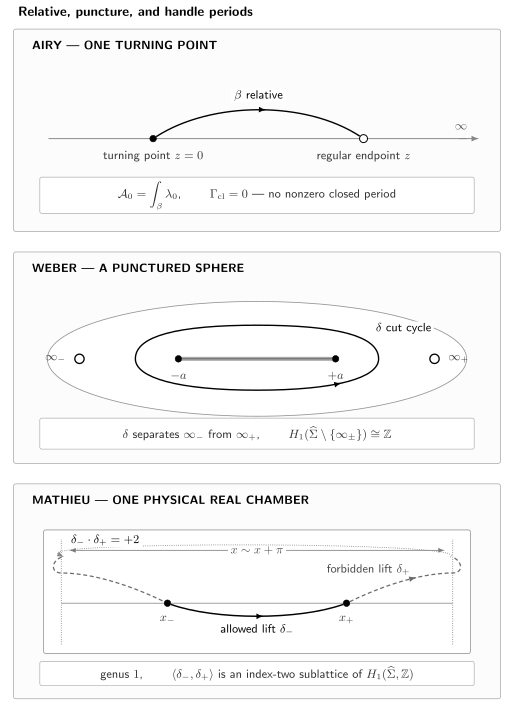
The examples separate relative-endpoint, puncture-loop, and handle data. For Mathieu, the physical cycles satisfy $\delta_-\mathbin{\cdot}\delta_+=2$ and span an index-two sublattice; a primitive basis has $A=\delta_-$ and $\delta_+=A+2B$.

The cover genus alone is therefore not a count of useful WKB quantities. One must also declare punctures, relative endpoints, and the differential being integrated.

Airy calibrates one simple turning point

Begin with the exact normal-form equation

$$\left[ -\hbar^2\partial_z^2+z \right]\psi=0, \qquad y^2=z.$$

The scaled coordinate

$$X=\frac{z}{\hbar^{2/3}}$$

turns it into $\psi_{XX}=X\psi$. Thus $\operatorname{Ai}(X)$ and $\operatorname{Bi}(X)$ are exact solutions. The scale $z=O(\hbar^{2/3})$ is already a warning: an ordinary WKB series at fixed $z$ cannot remain uniform as the turning point is approached.

On the branch $y=z^{1/2}$, Pages 2 and 5 found

$$\begin{aligned} \lambda_0 &= z^{1/2}\,\dd z, \\ \lambda_2 &= -\frac{5}{32z^{5/2}}\,\dd z. \end{aligned}$$

The compact cover is a sphere, so there is no nonzero closed classical period. The intrinsic half-contour prescription nevertheless gives the regularized action to a fixed ordinary point:

$$\mathcal A_{\mathrm{Ai}}^{\mathrm{reg}}(z,\hbar) = \frac23z^{3/2} + \frac{5\hbar^2}{48z^{3/2}} + O\!\left( \frac{\hbar^4}{z^{9/2}} \right).$$

For $\hbar>0$, take principal powers with $-\pi<\arg z<\pi$. As $|z|/\hbar^{2/3}\to\infty$, uniformly for $|\arg z|\leq\pi-\delta$, the standard Airy asymptotic expansion begins

$$\begin{aligned} \operatorname{Ai}\!\left( \frac{z}{\hbar^{2/3}} \right) \sim{}& \frac{\hbar^{1/6}}{2\sqrt\pi\,z^{1/4}} \exp\!\left[ -\frac{2z^{3/2}}{3\hbar} \right] \\ &\times \left[ 1- \frac{5\hbar}{48z^{3/2}} + O\!\left( \frac{\hbar^2}{z^3} \right) \right]. \end{aligned}$$

The decaying formal solution from Page 2 has the structure

$$P_{\mathrm{even}}^{-1/2} \exp\!\left[ -\frac{1}{\hbar} \mathcal A_{\mathrm{Ai}}^{\mathrm{reg}} \right].$$

Its order-$\hbar$ correction is exactly $-5\hbar/(48z^{3/2})$. The remaining factor $\hbar^{1/6}/(2\sqrt\pi)$ is an exact-solution normalization, not a period coefficient. This comparison fixes the sign and the half-contour normalization, but it does not provide a global connection formula: the displayed Airy expansion changes character when its sector boundary is crossed.

Near a generic simple turning point $z_t$, write $R_0(z)=c(z-z_t)+O((z-z_t)^2)$ with $c\neq0$. The local variable

$$X = \frac{c^{1/3}(z-z_t)}{\hbar^{2/3}}$$

reduces the leading equation to Airy form. Airy is therefore a local normal form for each isolated simple turning point, not a global model for a curve with several cycles.

Weber keeps closed and relative information separate

Take the harmonic-oscillator equation

$$\left[ -\hbar^2\partial_z^2+z^2 \right]\psi = a^2\psi, \qquad a>0.$$

Its WKB curve is $y^2=z^2-a^2$. The two finite turning points are $z=\pm a$, while the two points $\infty_\pm$ above infinity are unramified poles of $\lambda_0=y\,\dd z$. Fix their sheet labels by

$$\frac yz\longrightarrow\pm1 \qquad \text{at }\infty_\pm.$$

Let $\delta$ be the positively oriented lift of the cut from $-a$ to $a$ in the orientation fixed on Page 4. Residue evaluation gives

$$\Pi_{\delta,0} = \ii\pi a^2.$$

Every higher even Weber differential is residue-free. On the punctured genus-zero cover it is therefore exact, so the complete closed formal period truncates:

$$\Pi_\delta^{\mathrm{form}}(\hbar) = \ii\pi a^2, \qquad \Pi_{\delta,2k}=0 \quad(k\geq1).$$

The first exactness certificate is concrete:

$$\lambda_2 = \dd\!\left( \frac{5z}{24y^3} - \frac{z}{24a^2y} \right).$$

Its primitive returns to the same value around $\delta$ but has different finite parts at the two points over infinity.

This does not make all higher Weber data zero. For the relative path $\beta:\infty_-\to\infty_+$ used on Page 5, define

$$W_\beta^{\mathrm{form}}(\hbar) := \frac1\hbar \int_\beta \left( \Omega-\lambda_0 \right).$$

Define the Bernoulli polynomials by

$$\frac{s e^{xs}}{e^s-1} = \sum_{n\geq0} B_n(x)\frac{s^n}{n!}.$$

The endpoint values give the complete series

$$\begin{aligned} W_\beta^{\mathrm{form}}(\hbar) &= \sum_{k\geq1} \frac{B_{2k}(1/2)}{(2k-1)(2k)} \left( \frac{2\hbar}{a^2} \right)^{2k-1} \\ &= \sum_{k\geq1} \frac{ \left(1-2^{2k-1}\right)B_{2k} }{ 2k(2k-1) } \frac{ \hbar^{2k-1} }{ a^{4k-2} }. \end{aligned}$$

Here $B_n:=B_n(0)$, and the second line uses $B_n(1/2)=(2^{1-n}-1)B_n$.

The first terms are

$$\begin{aligned} W_\beta^{\mathrm{form}} ={}& -\frac{\hbar}{12a^2} + \frac{7\hbar^3}{360a^6} \\ & - \frac{31\hbar^5}{1260a^{10}} + O(\hbar^7). \end{aligned}$$

Thus the same exact differentials that disappear on $\delta$ retain nonzero endpoint constants on $\beta$.

The exact special function makes the all-orders formula transparent. Put

$$t=\frac{a^2}{2\hbar}.$$

After the scaling $X=\sqrt{2/\hbar}\,z$, the equation becomes

$$\begin{aligned} \frac{\dd^2\psi}{\dd X^2} + \left( \nu+\frac12-\frac{X^2}{4} \right)\psi &=0, \\ \nu &=t-\frac12. \end{aligned}$$

whose standard solutions include $D_\nu(X)$. Parabolic-cylinder connection coefficients contain gamma functions. Removing the elementary Stirling part gives

$$\begin{aligned} G(t) :={}& \log\Gamma\!\left(t+\frac12\right) \\ &{}-t\log t+t -\frac12\log(2\pi), \\ G(t) \sim{}& W_\beta^{\mathrm{form}}(\hbar), \qquad t\to\infty, \end{aligned}$$

with compatible logarithm branches and in a Stirling sector. This is an asymptotic comparison, not an assertion that a divergent formal series equals an analytic function without a summation prescription.

The exact spectrum is a benchmark, not a formal corollary

For the real-line oscillator, a solution decaying at both infinities exists precisely when $\nu=n\in\mathbb Z_{\geq0}$. Hence

$$a_n^2 = (2n+1)\hbar.$$

Equivalently, the positive mechanical action $J=-\ii\Pi_{\delta,0}=\pi a^2$ obeys

$$J = 2\pi\hbar \left(n+\frac12\right).$$

The numerical equality is exact for this quadratic potential, but its logical source is the two-ended boundary condition encoded by the parabolic-cylinder connection coefficient. The formal closed period alone does not manufacture the half-integer shift. Chapter 9 will derive how local turning-point connection data and global boundary conditions enter a quantization condition.

Mathieu turns the periodic cylinder into a torus

Use the periodic Schrödinger convention with $\Lambda>0$:

$$\begin{aligned} \left[ -\hbar^2\partial_x^2 +V(x) \right]\psi &=E\psi, \\ V(x) &=2\Lambda^2\cos(2x). \end{aligned}$$

The standard Mathieu parameters are

$$a_{\mathrm M} = \frac{E}{\hbar^2}, \qquad q_{\mathrm M} = \frac{\Lambda^2}{\hbar^2}.$$

Thus the semiclassical limit at fixed $E$ and $\Lambda$ is a correlated large-$a_{\mathrm M}$, large-$q_{\mathrm M}$ limit. It is not the small-$q_{\mathrm M}$ perturbation theory tabulated for weak periodic potentials.

Set $w=\exp(2\ii x)$. Then

$$R_0 = \Lambda^2\left(w+w^{-1}\right)-E.$$

With $Y=wy$, the compact spectral curve and its action differential are

$$\begin{aligned} Y^2 &= w\left( \Lambda^2w^2-Ew+\Lambda^2 \right), \\ \lambda_0 &= \frac{Y}{2\ii w^2}\,\dd w, \\ \partial_E\lambda_0 &= -\frac{\dd w}{4\ii Y}. \end{aligned}$$

This is a compactification of the classical curve. Substituting $w=\exp(2\ii x)$ directly into the quantum equation creates a first derivative; returning that equation to normal form requires the half-density and Schwarzian transformation developed on Page 8.

The four branch points are $0$, $\infty$, and

$$w_\pm = \frac{ E\pm\sqrt{E^2-4\Lambda^4} }{2\Lambda^2}, \qquad w_+w_-=1.$$

For $E\neq\pm2\Lambda^2$ they are distinct, and the compact cover has genus one. The two finite discriminant values are the minimum and maximum of the real potential. The form $\lambda_0$ has second-kind poles at the ramification points over $w=0$ and $w=\infty$; these are the two complex ends of the cylinder. The handle cycles used below avoid them.

Real Mathieu cycles reduce to complete elliptic integrals

Assume temporarily that

$$-2\Lambda^2<E<2\Lambda^2$$

and define the elliptic parameter

$$m := \frac{E+2\Lambda^2}{4\Lambda^2}, \qquad 0<m<1.$$

To avoid confusing a modulus with a parameter, use

$$\begin{aligned} \mathbf K(m) &:= \int_0^{\pi/2} \frac{\dd\theta}{ \sqrt{1-m\sin^2\theta}}, \\ \mathbf E(m) &:= \int_0^{\pi/2} \sqrt{1-m\sin^2\theta}\,\dd\theta. \end{aligned}$$

The two turning points bounding the allowed interval can be represented in the physical cell by

$$x_\pm = \frac\pi2 \pm\arcsin\sqrt m \pmod{\pi}.$$

First keep the two physical real contours distinct from a canonical basis. Let $\delta_-$ be the doubled allowed interval around the minimum at $x=\pi/2$, and let $\delta_+$ be the doubled forbidden interval across the maximum at $x=0$. In the convention $y^2=V-E$, orient them so that

$$\begin{aligned} \Pi_{\delta_-,0} &= \ii J_-, \\ \Pi_{\delta_+,0} &= J_+. \end{aligned}$$

The positive real actions are

$$\begin{aligned} J_- &= 8\Lambda \left[ \mathbf E(m) -(1-m)\mathbf K(m) \right], \\ J_+ &= 8\Lambda \left[ \mathbf E(1-m) -m\mathbf K(1-m) \right]. \end{aligned}$$

Both $\delta_-$ and $\delta_+$ are primitive, but they are not a symplectic pair. After their common branch-point endpoints are resolved, the two crossings have the same sign. Choose the global cycle orientations so that this sign is positive. Each resolved crossing then contributes $+1$, giving

$$\delta_-\mathbin{\cdot}\delta_+=+2.$$

Equivalently, the complementary base arcs join to a loop around the branch point $w=0$. This is the cylinder’s two-ended topology made visible on the double cover. A primitive integral basis can be chosen so that

$$\begin{aligned} A &=\delta_- , \\ \delta_+ &=A+2B, \\ A\mathbin{\cdot}B &=+1. \end{aligned}$$

Consequently, the corresponding primitive-basis periods are

$$\Pi_{A,0}=\ii J_- , \qquad \Pi_{B,0} = \frac{J_+-\ii J_-}{2}.$$

Although the last expression contains $1/2$, $B$ is an integral cycle: the two real vanishing cycles represent the same class modulo $2$ on this four-branch-point cover.

The derivative check is particularly simple for the physical actions:

$$\partial_EJ_- = \frac{\mathbf K(m)}{\Lambda}, \qquad \partial_EJ_+ = -\frac{\mathbf K(1-m)}{\Lambda}.$$

In the primitive basis this implies

$$\begin{aligned} \partial_E\Pi_{A,0} &= \frac{\ii\mathbf K(m)}{\Lambda}, \\ \partial_E\Pi_{B,0} &= -\frac{ \mathbf K(1-m)+\ii\mathbf K(m) }{2\Lambda}. \end{aligned}$$

The resulting elliptic ratio is a useful orientation check:

$$\begin{aligned} \tau :={}& \frac{\partial_E\Pi_{B,0}}{ \partial_E\Pi_{A,0}} \\ &= -\frac12 + \frac{\ii\mathbf K(1-m)}{2\mathbf K(m)}, \\ \operatorname{Im}\tau &>0. \end{aligned}$$

As $E\to-2\Lambda^2$, $\delta_-=A$ collapses around the potential minimum. As $E\to+2\Lambda^2$, $\delta_+=A+2B$ collapses around the maximum. Analytic continuation away from the real chamber transports the integral cycle lattice; it does not preserve the labels “allowed” and “forbidden.”

One operator computes both Mathieu quantum periods

Let

$$R_0(x;E) = 2\Lambda^2\cos(2x)-E, \qquad y^2=R_0.$$

The action form has the exact Picard–Fuchs certificate

$$\begin{aligned} &\left[ \left(E^2-4\Lambda^4\right)\partial_E^2 + \frac14 \right]\lambda_0 \\ &\qquad= \dd_x\!\left[ \frac{\Lambda^2\sin(2x)}{2y} \right]. \end{aligned}$$

Therefore every flat closed period satisfies

$$\left[ \left(E^2-4\Lambda^4\right)\partial_E^2 + \frac14 \right] \Pi_{\gamma,0} =0.$$

The leading coefficient vanishes at exactly the two finite discriminant values. The elliptic formulas above solve this equation with different cycle data.

For the source-free equation, direct substitution in the Page 6 formula for $\lambda_2$ gives the pointwise identity

$$\begin{aligned} \lambda_2 ={}& \left[ -\frac14\partial_E -3E\partial_E^2 \right. \\ &\left. \qquad -\frac53 \left(E^2-4\Lambda^4\right) \partial_E^3 \right] \lambda_0. \end{aligned}$$

Reducing the third derivative by the Picard–Fuchs equation gives, for every flat closed cycle $\gamma$,

$$\begin{aligned} \Pi_{\gamma,2} &= \left[ \frac16\partial_E + \frac E3\partial_E^2 \right] \Pi_{\gamma,0} \\ &= \left[ \frac16\partial_E - \frac{E}{ 12\left(E^2-4\Lambda^4\right) } \right] \Pi_{\gamma,0}. \end{aligned}$$

The second representative is valid only off the discriminant. Acting first on the two physical real periods gives

$$\begin{aligned} \Pi_{\delta_-,2} &= \ii J_{-,2}, \\ \Pi_{\delta_+,2} &= J_{+,2}. \end{aligned}$$

Here

$$\begin{aligned} J_{-,2} &:= \frac{\mathbf K(m)}{12\Lambda m} \\ &\quad+ \frac{ (2m-1)\mathbf E(m) }{12\Lambda m(1-m)}, \\ J_{+,2} &:= -\frac{\mathbf K(1-m)}{12\Lambda(1-m)} \\ &\quad+ \frac{ (2m-1)\mathbf E(1-m) }{12\Lambda m(1-m)}. \end{aligned}$$

Linearity then preserves the integral normalization:

$$\Pi_{A,2} = \ii J_{-,2}, \qquad \Pi_{B,2} = \frac{J_{+,2}-\ii J_{-,2}}{2}.$$

These are formal coefficients, not Borel sums. As a cycle degeneration is approached, the first correction has a finite one-sided limit while the corresponding classical action vanishes:

$$\begin{aligned} m\to0: \quad J_- &\sim2\pi\Lambda m, \\ J_{-,2} &\to\frac{\pi}{16\Lambda}, \\ m\to1: \quad J_+ &\sim2\pi\Lambda(1-m), \\ J_{+,2} &\to-\frac{\pi}{16\Lambda}. \end{aligned}$$

Thus $\hbar^2J_{\pm,2}$ is no longer a small correction relative to $J_\pm$; fixed-energy WKB is nonuniform there. For example, near the minimum put $x=\pi/2+u$ and $E=-2\Lambda^2+\epsilon$. Then

$$2\Lambda^2\cos(2x)-E = 4\Lambda^2u^2-\epsilon +O(u^4),$$

so a correlated local scaling produces the Weber problem. At an isolated turning point away from the collision, the local model is Airy. The three examples are therefore nested rather than unrelated.

Floquet data require the analytic layer

Mathieu’s exact solutions may be normalized by

$$\psi(x+\pi) = \exp(\ii\pi\nu)\psi(x),$$

where $\nu$ is the characteristic exponent. Periodic and antiperiodic band edges correspond to integral $\nu$. The formal $A$- and $B$-periods are ingredients in semiclassical descriptions of this monodromy, but the equation above is an exact statement about an analytic solution. Converting the formal periods into its exact Hill discriminant requires a summation chamber, Stokes data, and a global connection formula. Those enter Chapter 9; the band spectrum is developed in Chapter 14.

Reproducible three-model audit

The Airy–Weber–Mathieu check verifies:

• the Airy scaling, first even WKB correction, and asymptotic coefficient;
• Weber closed residues and several terms of the Bernoulli formula;
• the Weber gamma-tail coefficients and parabolic-cylinder parameter;
• the Mathieu algebraic curve, discriminant, Picard–Fuchs certificate, and first quantum operator;
• the real $J_-$ and $J_+$ actions against direct quadrature, followed by the primitive-basis conversion.

Run

python3 public/code/advanced-ode/airy-weber-mathieu-check.py

The script checks formal identities and a high-precision classical quadrature. It does not Borel-sum a series, determine a Stokes chamber, or solve a Mathieu band problem.

Common pitfalls

Dropping the imaginary unit in an allowed region. With $y^2=V-E$, the chosen momentum is imaginary where $E>V$. Convert to the positive mechanical action only after fixing the sheet and cycle orientation.

Treating Airy asymptotics as one global formula. The exact Airy function is entire, but each displayed asymptotic representation has a sector. Continuing the exact function and continuing one formal expansion are not the same operation.

Calling every Weber correction zero. Higher closed periods vanish, whereas the pole-to-pole correction has a nontrivial Bernoulli series. The difference is absolute versus relative data, not a contradiction.

Deriving the Maslov shift from a classical integral alone. The closed Weber action happens to reproduce the exact energies after a half-integer condition is supplied. The shift comes from analytic turning-point and boundary data.

Confusing Mathieu’s parameter with the cylinder coordinate. The standard parameter is $q_{\mathrm M}=\Lambda^2/\hbar^2$; the algebraic coordinate used above is $w=\exp(2\ii x)$. They play unrelated roles.

Substituting a discriminant value into a regular-family operator. At $E=\pm2\Lambda^2$, a cycle degenerates and the fixed-energy WKB expansion is nonuniform. Coefficientwise endpoint limits can diagnose the failure, but spectral conclusions at the colliding pair require a Weber scaling. Airy applies while an individual turning point remains isolated.

Exercises

1. Match the first Airy correction

Starting from the regularized Airy action, expand

$$z^{-1/4} \exp\!\left[ -\frac1\hbar \mathcal A_{\mathrm{Ai}}^{\mathrm{reg}} \right]$$

through relative order $\hbar$. Compare it with the first correction in the asymptotic expansion of $\operatorname{Ai}(z/\hbar^{2/3})$.

Solution

Substitution gives

$$\begin{aligned} &z^{-1/4} \exp\!\left[ -\frac{2z^{3/2}}{3\hbar} - \frac{5\hbar}{48z^{3/2}} +O(\hbar^3) \right] \\ &\qquad= z^{-1/4} \exp\!\left[ -\frac{2z^{3/2}}{3\hbar} \right] \\ &\qquad\quad\times \left[ 1- \frac{5\hbar}{48z^{3/2}} +O(\hbar^2) \right]. \end{aligned}$$

This is the first Airy coefficient. The exact normalization $\hbar^{1/6}/(2\sqrt\pi)$ is independent of $z$ and is not fixed by the phase integral.

2. Reduce Weber to parabolic-cylinder form

Apply $X=\sqrt{2/\hbar}\,z$ to the Weber equation and derive $\nu=a^2/(2\hbar)-1/2$. Explain why decay at both real infinities forces $\nu$ to be a nonnegative integer.

Solution

Since $\partial_z^2=(2/\hbar)\partial_X^2$, division by $2\hbar$ gives

$$\frac{\dd^2\psi}{\dd X^2} + \left[ \frac{a^2}{2\hbar} - \frac{X^2}{4} \right]\psi =0.$$

Comparison with the standard equation identifies $\nu+1/2=a^2/(2\hbar)$. The solution $D_\nu(X)$ decays for $X\to+\infty$. Its connection formula at $-\infty$ contains a growing component proportional to $1/\Gamma(-\nu)$. That coefficient vanishes exactly for $\nu=n\in\mathbb Z_{\geq0}$, giving $a_n^2=(2n+1)\hbar$.

3. Recover the Weber Bernoulli coefficients

Use the shifted Stirling expansion of $\log\Gamma(t+1/2)$ to compute the first three inverse powers in $G(t)$. Substitute $t=a^2/(2\hbar)$.

Solution

The shifted expansion is

$$\begin{aligned} G(t) \sim{}& -\frac{1}{24t} + \frac{7}{2880t^3} \\ & - \frac{31}{40320t^5} + O(t^{-7}). \end{aligned}$$

Since $t^{-(2k-1)}=(2\hbar/a^2)^{2k-1}$, this becomes

$$-\frac{\hbar}{12a^2} + \frac{7\hbar^3}{360a^6} - \frac{31\hbar^5}{1260a^{10}} + O(\hbar^7),$$

which is the pole-to-pole series. It says nothing about the higher closed periods, which vanish separately.

4. Derive the real Mathieu actions

For $-2\Lambda^2<E<2\Lambda^2$, derive $J_-$ by writing $x=\pi/2+u$ and then setting $\sin u=\sqrt m\sin\theta$. Obtain $J_+$ by the complementary substitution around $x=0$.

Solution

Around the minimum,

$$E-2\Lambda^2\cos(2x) = 4\Lambda^2 \left( m-\sin^2u \right).$$

The doubled allowed action is therefore

$$J_- = 8\Lambda \int_0^{\arcsin\sqrt m} \sqrt{m-\sin^2u}\,\dd u.$$

The stated substitution reduces the integral to $\mathbf E(m)-(1-m)\mathbf K(m)$. Around the maximum,

$$2\Lambda^2\cos(2x)-E = 4\Lambda^2 \left( 1-m-\sin^2x \right),$$

and the same calculation with $m\mapsto1-m$ gives $J_+=8\Lambda[\mathbf E(1-m)-m\mathbf K(1-m)]$.

5. Recover a primitive Mathieu basis

Suppose the oriented real vanishing cycles obey $\delta_-\mathbin{\cdot}\delta_+=2$ and choose $A=\delta_-$, $\delta_+=A+2B$. Verify the intersection of $A$ and $B$, and express their classical periods in terms of $J_-$ and $J_+$.

Solution

Skew-symmetry gives $A\mathbin{\cdot}A=0$, so

$$2 = \delta_-\mathbin{\cdot}\delta_+ = A\mathbin{\cdot}(A+2B) = 2A\mathbin{\cdot}B.$$

Hence $A\mathbin{\cdot}B=1$. Periods are linear in homology, and the chosen real-cycle orientations give

$$\Pi_{A,0}=\ii J_- , \qquad \Pi_{B,0} = \frac{J_+-\ii J_-}{2}.$$

The division by two occurs in a change between integral bases; it does not license arbitrary half-integral cycles.

6. Verify the Mathieu Picard–Fuchs certificate

For $R_0=2\Lambda^2\cos(2x)-E$, prove the exact-form identity in the text and integrate it over a flat closed cycle.

Solution

Because $\partial_E^2\lambda_0=-\dd x/(4y^3)$, the left-hand side has coefficient

$$-\frac{E^2-4\Lambda^4}{4y^3} + \frac y4.$$

Use $y^2=2\Lambda^2\cos(2x)-E$ to put this over $y^3$. Differentiating $\Lambda^2\sin(2x)/(2y)$ gives the same numerator. The primitive is single-valued meromorphic on the spectral cover, so its integral over a closed cycle vanishes.

7. Reduce the first Mathieu operator

Starting from the third-order pointwise operator for $\lambda_2$, differentiate the Picard–Fuchs equation once and derive the second-order period operator.

Solution

Let $D=E^2-4\Lambda^4$ and let $f$ be a classical period. Then

$$\begin{aligned} Df''+\frac14f &=0, \\ Df'''+2Ef''+\frac14f' &=0. \end{aligned}$$

Substitution in

$$-\frac14f' -3Ef'' -\frac53Df'''$$

gives

$$\frac16f' + \frac E3f''.$$

Using the first Picard–Fuchs equation once more yields the equivalent first-order representative

$$\frac16f' - \frac{E}{12D}f.$$

Its discriminant pole is introduced by derivative-order reduction.

8. Identify the two Mathieu local models

Expand the potential near $x=\pi/2$ and $x=0$. Which local equation appears when the energy approaches the corresponding extremum? What model applies at one isolated turning point before the collision?

Solution

With $x=\pi/2+u$,

$$2\Lambda^2\cos(2x) = -2\Lambda^2+4\Lambda^2u^2+O(u^4).$$

Near $x=0$,

$$2\Lambda^2\cos(2x) = 2\Lambda^2-4\Lambda^2x^2+O(x^4).$$

The lower collision is an ordinary Weber oscillator and the upper collision is its inverted continuation. Away from either collision, each individual simple turning point has an Airy scaling. The elliptic expansion must be reorganized in the correlated local limit: a finite coefficientwise endpoint limit does not make the fixed-energy WKB hierarchy uniform there.

References

• NIST Digital Library of Mathematical Functions, §9.2 and §9.7(ii), equation (9.7.5). Defines the Airy equation and gives the sectorial Poincaré expansion used for the normalization check.
• NIST Digital Library of Mathematical Functions, equation (12.2.4), equation (12.2.5), §12.2(v), equation (12.7.2), and §12.9(i). Defines $D_\nu$, records the connection formulas, identifies the Hermite-polynomial cases, and supplies the large-variable asymptotics used in the oscillator benchmark.
• NIST Digital Library of Mathematical Functions, §5.11(i). Gives Stirling expansions and their sector conditions for the gamma-function comparison.
• K. Iwaki, T. Koike, and Y.-M. Takei, “Voros Coefficients for the Hypergeometric Differential Equations and Eynard–Orantin’s Topological Recursion, Part I: For the Weber Equation”, Annales Henri Poincaré 24 (2023), 1305–1353, §4, especially Theorem 4.10. Derives the complete Weber Voros coefficient in terms of Bernoulli polynomials. Its normalization maps to this page by $x_{\mathrm{IKT}}=2z$, $\hbar_{\mathrm{IKT}}=2\hbar$, $\lambda_{\mathrm{IKT}}=a^2$, and $\nu_{\mathrm{IKT}}=0$; its rational-cover path $0\to\infty$ represents the oriented path $\infty_-\to\infty_+$ used here.
• NIST Digital Library of Mathematical Functions, §28.2(i), equations (28.2.1)–(28.2.3), §28.2(iii), equations (28.2.14)–(28.2.16), and §28.2(v), especially Table 28.2.1. Fixes the standard Mathieu parameters, algebraic forms, and Floquet normalization, including the periodic and antiperiodic integral characteristic exponents.
• NIST Digital Library of Mathematical Functions, §19.2(ii) and §19.4(i). Defines the complete elliptic integrals and records the derivative identities used for $J_-$ and $J_+$; the DLMF modulus satisfies $k^2=m$ here.
• K. Imaizumi, “Exact WKB Analysis and TBA Equations for the Mathieu Equation”, Physics Letters B 806 (2020), 135500, §§2–3, especially equations (2.1)–(2.12) and (3.16)–(3.18). Gives the two Mathieu cycle sectors and the first quantum-period operator; Figure 2.1 and equations (2.13)–(2.14) also display the two same-sign crossings behind the physical-cycle factor $2$. Its variables translate by $q=2x$, $\hbar_{\mathrm{there}}=2\hbar$, and $\Lambda_{\mathrm{there}}^2=2\Lambda^2$, with $u_{\mathrm{there}}=E$ and $p_{\mathrm{there}}^2=E-V=-y^2$. On the selected sheet its period is $a_{\mathrm{there}}=-2\ii\Pi_{\mathrm{here}}$, and the first operator rescales as $\mathcal D_{\mathrm{here}}=4\mathcal D_{1,\mathrm{there}}$, giving $\frac16\partial_E+\frac E3\partial_E^2$. Imaizumi draws the cycles on $q\sim q+4\pi$; the degree-two quotient to $q\sim q+2\pi$, equivalently this page’s $x\sim x+\pi$, identifies his equal-period forbidden cycles $\beta$ and $\widetilde\beta$ while retaining their two same-sign crossings.
• A.-K. Kashani-Poor and J. Troost, “Pure $\mathcal N=2$ Super Yang–Mills and Exact WKB”, Journal of High Energy Physics 08 (2015), 160, §2.1. Uses an intersection-one homology basis for the same elliptic curve–Mathieu correspondence, providing the primitive-basis side of the cycle normalization used here.
• J. L. Dunham, “The Wentzel–Brillouin–Kramers Method of Solving the Wave Equation”, Physical Review 41 (1932), 713–720. Classical source for the all-orders closed-contour expansion and oscillator benchmark.