Local Exponents, Masses, and Liouville Momenta

A regular $A_1$ puncture carries one Cartan mass, but it appears under several different names. A localization formula prints a frame-dependent hypermultiplet mass. A Liouville block uses a dimensionless momentum. A degenerate OPE sees an ordered difference of fusion powers. A normal-form ODE retains its square through a double-pole coefficient, and a monodromy trace forgets still more information. Equating any two of these labels without the intermediate shifts and branches is a common source of correct-looking but incompatible dictionaries.

This page makes the regular-puncture chain reversible. The book keeps $b^2=\epsilon_2/\epsilon_1$, so the light field $V_{-b/2}$ measures $2p/\epsilon_1$ and survives the $\epsilon_2\to0$ NS limit. Exchanging the Omega planes measures $2p/\epsilon_2$ with the dual degenerate field. That exchange preserves the central charge and conformal weight, but it does not preserve the same semiclassical problem.

First pass

Read the one-puncture ladder, the four-flavor mass table, and the Heun reverse algorithm. The monodromy and exceptional-locus sections explain why squared or traced data cannot determine a signed mass by themselves.

Status ledger

Statement used on this page	Status
$p_f\leftrightarrow\alpha_f$ and the four-flavor affine mass map	Exact algebra in the declared regular $A_1$ AGT representative
The two fusion powers of $V_{-b/2}$ or $V_{-1/(2b)}$	Exact Virasoro OPE data after the degenerate quotient and fusion rule are imposed
A degenerate insertion is represented by the defect of Page 4	Physical AGT proposal; separately, the displayed tuned partition function obeys an exact model-specific localization Ward identity
The NS remainder has the printed oper exponents	Conditional on the connected, derivative-compatible factorization and normalization fixed on Pages 2 and 4
A conformal weight or oper double pole determines an oriented mass	False; both are invariant under Liouville or puncture Weyl reflection
A monodromy trace determines one exponent difference	False without an $SL(2)$ lift, eigenvalue ordering, and logarithm branch
Integer exponent difference forces a logarithm	False; it permits a logarithm, whose coefficient is a separate local obstruction
The regular-puncture table applies unchanged after confluence	False; an irregular end requires formal exponential, formal monodromy, and Stokes data

External, internal, and degenerate momenta occupy different slots

Before writing formulas, separate the roles of three CFT momenta:

Momentum slot	Surface datum	Gauge datum	ODE role
External $\alpha_f$	A regular marked point	Centered puncture mass $p_f$	Local exponent difference at an endpoint
Internal $\alpha_{0t}$	The tube in the $0t$ sewing channel	Coulomb modulus $a_{\mathrm C}$	Composite monodromy or channel datum, not a fifth endpoint mass
Degenerate momentum	A moving null-state probe	Defect polarization and vacuum	Selects the BPZ operator and which Omega plane supplies its exponent coordinate

This page concerns the first row and the probe that reads it. Page 6 develops the internal row. The irregular-puncture page explains why a confluent endpoint no longer has only two Frobenius powers.

Fix compatible square-root branches by

$$\begin{gathered} \varepsilon_\star^2 = \epsilon_1\epsilon_2, \qquad b^2 = \frac{\epsilon_2}{\epsilon_1}, \\ \varepsilon_\star = b\epsilon_1 = \frac{\epsilon_2}{b}, \qquad Q_{\mathrm L} = b+b^{-1} = \frac{\epsilon_\Sigma}{\varepsilon_\star}, \end{gathered}$$

where $\epsilon_\Sigma=\epsilon_1+\epsilon_2$. A centered, dimensionful puncture mass $p_f$ and its unreflected Liouville representative are related by

$$\alpha_f = \frac{Q_{\mathrm L}}2 + \frac{p_f}{\varepsilon_\star}, \qquad p_f = \varepsilon_\star \left( \alpha_f-\frac{Q_{\mathrm L}}2 \right).$$

The conformal weight is therefore

$$\begin{aligned} \Delta_f &= \alpha_f \left( Q_{\mathrm L}-\alpha_f \right) \\ &= \frac{Q_{\mathrm L}^2}{4} - \frac{p_f^2}{\epsilon_1\epsilon_2} \\ &= \frac{ \epsilon_\Sigma^2-4p_f^2 }{ 4\epsilon_1\epsilon_2 }. \end{aligned}$$

The map $p_f\mapsto\alpha_f$ is one-to-one after the branches and reflection representative are fixed. The map $\alpha_f\mapsto\Delta_f$ is generically two-to-one; its branches meet at $\alpha_f=Q_{\mathrm L}/2$.

The ordered Omega pair produces two exponent coordinates

There are two level-two degenerate probes. It is useful to name the oriented differences they measure before taking either semiclassical limit:

$$\begin{aligned} \theta_f^{[1]} &:= 2b \left( \alpha_f-\frac{Q_{\mathrm L}}2 \right) = \frac{2p_f}{\epsilon_1}, \\ \theta_f^{[2]} &:= \frac{2}{b} \left( \alpha_f-\frac{Q_{\mathrm L}}2 \right) = \frac{2p_f}{\epsilon_2}. \end{aligned}$$

Page 2’s $\theta_f$ is $\theta_f^{[1]}$. The superscript records the Omega plane whose equivariant weight appears in the denominator; it is not a tensor index.

Probe	Null relation	Fusion channels	Difference and inverse
$V_{-b/2}$	$(L_{-1}^2+b^2L_{-2})V_{-b/2}=0$	$\alpha_f\mp b/2$	$\theta_f^{[1]}=2p_f/\epsilon_1$, $p_f=\epsilon_1\theta_f^{[1]}/2$
$V_{-1/(2b)}$	$(L_{-1}^2+b^{-2}L_{-2})V_{-1/(2b)}=0$	$\alpha_f\mp1/(2b)$	$\theta_f^{[2]}=2p_f/\epsilon_2$, $p_f=\epsilon_2\theta_f^{[2]}/2$

For a finite puncture and a local primary OPE trivialization, the exact fusion powers are

$$\begin{aligned} \rho_{f,\pm}^{[1]} &= \frac{ 1+b^2\pm\theta_f^{[1]} }{2}, \\ \rho_{f,\pm}^{[2]} &= \frac{ 1+b^{-2}\pm\theta_f^{[2]} }{2}. \end{aligned}$$

For example,

$$\begin{aligned} \Delta\left(\alpha_f-\frac b2\right) -\Delta(\alpha_f)-\Delta_{\mathrm d} &= b\alpha_f, \\ \Delta\left(\alpha_f+\frac b2\right) -\Delta(\alpha_f)-\Delta_{\mathrm d} &= b(Q_{\mathrm L}-\alpha_f), \end{aligned}$$

with $\Delta_{\mathrm d}=-1/2-3b^2/4$. Their ordered difference is $\theta_f^{[1]}$.

A scalar prefactor can shift both powers by the same number. Placement at infinity also requires the local coordinate $w=1/z$ and the half-density transformation. Thus the individual finite-$b$ powers are not portable without a trivialization, whereas their difference is. This explains the extra common $b^2/2$ shift in the left-chart powers printed on Page 4: their difference is still $\theta_\infty^{[1]}$, and their NS limits are the same unordered oper roots.

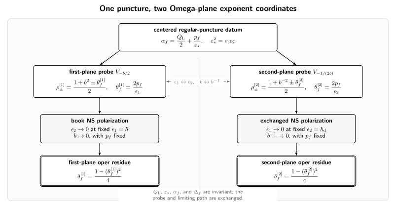
The ordered Omega pair creates two related, not identical, exponent dictionaries. The book’s $V_{-b/2}$ branch keeps $\theta_f^{[1]}=2p_f/\epsilon_1$ finite as $\epsilon_2\to0$. Exchanging the planes sends $b\leftrightarrow b^{-1}$, exchanges the two degenerate probes, and keeps $\theta_f^{[2]}=2p_f/\epsilon_2$ finite in the opposite limit. The conformal weight and central charge are invariant, but the light field and semiclassical path change together.

The NS path turns a fusion difference into an oper residue

The exact finite-Omega identities are

$$\begin{aligned} b^2\Delta_f &= \frac{ (1+b^2)^2-(\theta_f^{[1]})^2 }{4}, \\ b^{-2}\Delta_f &= \frac{ (1+b^{-2})^2-(\theta_f^{[2]})^2 }{4}. \end{aligned}$$

In particular, the finite-Omega quantity is not yet the oper residue:

$$b^2\Delta_f = \frac{1-(\theta_f^{[1]})^2}{4} +\frac{b^2}{2} +\frac{b^4}{4}.$$

In the book’s NS direction,

$$\epsilon_2\longrightarrow0, \qquad \epsilon_1=\hbar\ \text{fixed}, \qquad p_f\ \text{fixed},$$

one has $b\to0$ and

$$\theta_f := \theta_f^{[1]} = \frac{2p_f}{\hbar} \quad\text{fixed}.$$

For generic fixed $\theta_f$ with $\theta_f^2\neq1$, the background primary is heavy in conformal-weight scaling:

$$\alpha_f = \frac{Q_{\mathrm L}}2 + \frac{\theta_f}{2b},$$

and

$$\Delta_f \sim \frac{1-\theta_f^2}{4b^2}.$$

At $\theta_f=\pm1$ the leading classical weight vanishes, $\Delta_f=O(1)$, so this limit is nonuniform. In either case $V_{-b/2}$ is light. The double-pole coefficient becomes

$$\delta_f := \lim_{b\to0}b^2\Delta_f = \frac{1-\theta_f^2}{4}.$$

When the normalized NS factorization of Page 4 exists, the local oper has

$$T_{\mathrm{op}}(z) = \frac{\delta_f}{(z-z_f)^2} + O\left((z-z_f)^{-1}\right),$$

and its half-density powers are

$$\rho_{f,\pm}^{\mathrm{op}} = \frac{1\pm\theta_f}{2}.$$

The dual identity belongs to the exchanged limit $\epsilon_1\to0$ at fixed $\epsilon_2$. Merely replacing $b$ by $b^{-1}$ while retaining the book’s NS path mixes the two polarizations.

The path must also specify which masses stay fixed. Define centered localization masses

$$M_i := \mu_i-\frac{\epsilon_\Sigma}{2}.$$

Holding the puncture data means holding the $M_i$, or equivalently the $p_f$, fixed. Then, exactly,

$$\mu_i = M_i+\frac{\hbar}{2}+\frac{\epsilon_2}{2}.$$

Holding the printed $\mu_i$ fixed is a different finite-Omega path. Although it gives the same leading value of some NS exponents, it changes subleading mass and contact terms and can change a normalized coupling derivative.

Reflection and monodromy forget the orientation

Liouville reflection, puncture Weyl reflection, and reversal of the ordered exponent pair induce the same sign reversal on the local passport:

$$\alpha_f \longmapsto Q_{\mathrm L}-\alpha_f, \qquad p_f\longmapsto-p_f, \qquad \theta_f^{[k]}\longmapsto-\theta_f^{[k]}.$$

Neither $\Delta_f$ nor $\delta_f$ changes. From a double-pole coefficient alone one can recover only

$$\theta_f = \pm\sqrt{1-4\delta_f}.$$

They need not act identically on a normalized conformal block or a raw localization formula: reflection amplitudes, Abelian factors, and scalar prefactors can distinguish the global representatives.

Even monodromy does not remove every ambiguity. For a declared determinant-one lift, write

$$\operatorname{spec}(M_f) = \left\{ \sigma_f\ee^{\pi\ii\theta_f}, \sigma_f\ee^{-\pi\ii\theta_f} \right\}, \qquad \sigma_f\in\{+1,-1\}.$$

Then

$$\operatorname{tr}M_f = 2\sigma_f\cos(\pi\theta_f),$$

and an inverse requires

$$\theta_f = \pm \frac1\pi \arccos \left( \frac{\operatorname{tr}M_f}{2\sigma_f} \right) + 2n, \qquad n\in\mathbb Z.$$

The natural half-density Frobenius powers give $\sigma_f=-1$. A different $SL(2)$ lift can change that sign. A projective monodromy ratio retains only $\theta_f$ modulo $\theta_f\sim\pm\theta_f+\mathbb Z$. Therefore a trace is not a signed mass.

Four printed masses become four puncture masses only after pairing

Return to the weakly coupled $N_f=4$ representative of Page 2: $\mu_{1,2}$ are printed antifundamental masses and $\mu_{3,4}$ are printed fundamental masses. In terms of the centered $M_i$, the full puncture passport is

Puncture	Centered mass	Book exponent coordinate
$\infty$	$p_\infty=(M_1-M_2)/2$	$\theta_\infty=(\mu_1-\mu_2)/\epsilon_1$
$1$	$p_1=(M_1+M_2)/2$	$\theta_1=(\mu_1+\mu_2-\epsilon_\Sigma)/\epsilon_1$
$t$	$p_t=(M_3+M_4)/2$	$\theta_t=(\mu_3+\mu_4-\epsilon_\Sigma)/\epsilon_1$
$0$	$p_0=(M_3-M_4)/2$	$\theta_0=(\mu_3-\mu_4)/\epsilon_1$

Equivalently,

$$\begin{aligned} p_\infty &= \frac{\mu_1-\mu_2}{2}, & p_1 &= \frac{\mu_1+\mu_2-\epsilon_\Sigma}{2}, \\ p_t &= \frac{\mu_3+\mu_4-\epsilon_\Sigma}{2}, & p_0 &= \frac{\mu_3-\mu_4}{2}. \end{aligned}$$

The inverse map restores the equivariant centering:

$$\begin{aligned} \mu_1 &= \frac{\epsilon_\Sigma}{2} + \frac{\epsilon_1}{2} \left( \theta_1+\theta_\infty \right), \\ \mu_2 &= \frac{\epsilon_\Sigma}{2} + \frac{\epsilon_1}{2} \left( \theta_1-\theta_\infty \right), \\ \mu_3 &= \frac{\epsilon_\Sigma}{2} + \frac{\epsilon_1}{2} \left( \theta_t+\theta_0 \right), \\ \mu_4 &= \frac{\epsilon_\Sigma}{2} + \frac{\epsilon_1}{2} \left( \theta_t-\theta_0 \right). \end{aligned}$$

Thus the four $\mu_i$ are not four puncture labels one by one. They are an affine coordinate system on the four centered Cartan masses in one matter orientation and one weak-coupling frame.

For the matrix row in the final passport, define

$$\boldsymbol\mu = \begin{pmatrix} \mu_1\\ \mu_2\\ \mu_3\\ \mu_4 \end{pmatrix}, \qquad \boldsymbol p = \begin{pmatrix} p_\infty\\ p_1\\ p_t\\ p_0 \end{pmatrix}, \qquad \boldsymbol s_F = \frac12 \begin{pmatrix} 1\\ 1\\ 1\\ 1 \end{pmatrix},$$

and

$$A_F = \begin{pmatrix} 1&1&0&0\\ -1&1&0&0\\ 0&0&1&1\\ 0&0&1&-1 \end{pmatrix}.$$

Then $\boldsymbol\mu=A_F\boldsymbol p+\epsilon_\Sigma\boldsymbol s_F$. The subscript $F$ records this particular weak-coupling frame; a duality move changes the affine representative.

The reflection operations make the representative dependence visible:

Reflected puncture	Transformation of printed masses in this frame
$\infty$	$(\mu_1,\mu_2)\mapsto(\mu_2,\mu_1)$
$1$	$(\mu_1,\mu_2)\mapsto(\epsilon_\Sigma-\mu_2,\epsilon_\Sigma-\mu_1)$
$0$	$(\mu_3,\mu_4)\mapsto(\mu_4,\mu_3)$
$t$	$(\mu_3,\mu_4)\mapsto(\epsilon_\Sigma-\mu_4,\epsilon_\Sigma-\mu_3)$

The complement $\mu\mapsto\epsilon_\Sigma-\mu$ exchanges a printed fundamental and antifundamental contribution in the AGT localization convention. It can also change the Abelian or Heisenberg prefactor, so the reflected mass list must not be inserted into an unchanged raw $U(2)$ formula.

The defect source variables pass through the same passport

Page 4 used the source’s $U(2)$ arrays $\boldsymbol A_0,\ldots,\boldsymbol A_3$ and $\bar A_i=(A_{i,1}+A_{i,2})/2$. One unreflected representative of its four weights is shown below. The $\mu_i$ reconstructed later in this section are Page 2’s printed AGT mass coordinates, not raw entries of these arrays.

Puncture or channel	Centered source datum
$\infty$	$p_\infty=(A_{0,1}-A_{0,2})/2$
$1$	$p_1=\bar A_0-\bar A_2+\epsilon_1/2$
$t$	$p_t=\bar A_2-\bar A_3+\epsilon_\Sigma/2$
$0$	$p_0=(A_{3,1}-A_{3,2})/2$
internal $0t$ channel	$a_{\mathrm C}=(A_{2,1}-A_{2,2})/2$

The corresponding external Liouville momenta are

$$\begin{aligned} \alpha_\infty &= \frac{ \epsilon_\Sigma+A_{0,1}-A_{0,2} }{ 2\varepsilon_\star }, & \alpha_0 &= \frac{ \epsilon_\Sigma+A_{3,1}-A_{3,2} }{ 2\varepsilon_\star }, \\ \alpha_t &= \frac{ \bar A_2-\bar A_3+\epsilon_\Sigma }{ \varepsilon_\star }, & \alpha_1 &= \frac{ 2\bar A_0-2\bar A_2+2\epsilon_1+\epsilon_2 }{ 2\varepsilon_\star }. \end{aligned}$$

Two substitutions audit the asymmetric-looking weights on Page 4. If $d_t=\bar A_2-\bar A_3$ and $d_1=\bar A_0-\bar A_2$, then

$$\begin{aligned} \frac{ \epsilon_\Sigma^2-4p_t^2 }{ 4\epsilon_1\epsilon_2 } &= - \frac{ d_t(d_t+\epsilon_\Sigma) }{ \epsilon_1\epsilon_2 }, \\ \frac{ \epsilon_\Sigma^2-4p_1^2 }{ 4\epsilon_1\epsilon_2 } &= - \frac{ (2d_1+2\epsilon_1+\epsilon_2) (2d_1-\epsilon_2) }{ 4\epsilon_1\epsilon_2 }. \end{aligned}$$

The Page 2 printed masses in this representative are

$$\begin{aligned} \mu_1 &= A_{0,1}-\bar A_2 +\epsilon_1+\frac{\epsilon_2}{2}, & \mu_2 &= A_{0,2}-\bar A_2 +\epsilon_1+\frac{\epsilon_2}{2}, \\ \mu_3 &= \bar A_2-A_{3,2}+\epsilon_\Sigma, & \mu_4 &= \bar A_2-A_{3,1}+\epsilon_\Sigma. \end{aligned}$$

Substitution recovers all four $p_f$ above. Reflecting any $p_f$ produces an equally valid CFT weight, but it also changes the printed representative and, in general, the scalar prefactor. The internal row is recorded only to prevent it from being mistaken for another external mass; Page 6 supplies its monodromy and accessory roles.

A Heun equation gives exponent data before it gives masses

Put a standard Heun equation in the book’s puncture order $(0,t,1,\infty)$. Its oriented exponent differences are

$$\begin{aligned} \theta_0 &= 1-\gamma_{\mathrm H}, & \theta_1 &= 1-\delta_{\mathrm H}, \\ \theta_t &= 1-\epsilon_{\mathrm H}, & \theta_\infty &= \alpha_{\mathrm H}-\beta_{\mathrm H}. \end{aligned}$$

Here $\alpha_{\mathrm H},\beta_{\mathrm H}$ are Heun parameters, not Liouville momenta. The inverse exponent map is

$$\begin{aligned} \gamma_{\mathrm H} &= 1-\theta_0, & \delta_{\mathrm H} &= 1-\theta_1, & \epsilon_{\mathrm H} &= 1-\theta_t, \\ \alpha_{\mathrm H} &= \frac{ 2-\theta_0-\theta_1-\theta_t+\theta_\infty }{2}, \\ \beta_{\mathrm H} &= \frac{ 2-\theta_0-\theta_1-\theta_t-\theta_\infty }{2}. \end{aligned}$$

The final two rows automatically enforce the Heun Fuchs relation. A reverse ODE-to-gauge audit now has five steps:

1. Move the singularities to $(0,t,1,\infty)$ and record every scalar exponent gauge.
2. Extract the four oriented $\theta_f$ from the printed Heun parameters.
3. Choose $\epsilon_1,\epsilon_2$, compatible square-root branches, and the book’s NS polarization.
4. Recover $p_f=\epsilon_1\theta_f/2$, then $\alpha_f$ and the four $\mu_i$ from the formulas above.
5. Reinsert the result into the conformal weights and localization factors; separately flag every resonant endpoint.

This algorithm does not determine the accessory parameter. A scalar gauge that swaps an exponent can shift the standard Heun accessory even though it leaves the underlying local conjugacy class unchanged. That translation belongs to Page 6.

A rational round-trip check

Take

$$\epsilon_1=2, \qquad \epsilon_2=\frac12, \qquad \theta_0=\frac13, \qquad \theta_t=-\frac25.$$

Then

$$b=\frac12, \qquad \varepsilon_\star=1, \qquad Q_{\mathrm L}=\frac52,$$

and the right flavor pair is

$$\begin{aligned} p_0&=\frac13, & p_t&=-\frac25, \\ \mu_3&=\frac{71}{60}, & \mu_4&=\frac{31}{60}. \end{aligned}$$

At the puncture $0$,

$$\alpha_0=\frac{19}{12}, \qquad \left( \rho_{0,+}^{[1]}, \rho_{0,-}^{[1]} \right) = \left( \frac{19}{24}, \frac{11}{24} \right).$$

Their difference is $1/3$, while

$$\Delta_0 = \frac{209}{144}, \qquad b^2\Delta_0 = \rho_{0,+}^{[1]}\rho_{0,-}^{[1]} = \frac{209}{576}.$$

The NS oper residue is instead

$$\delta_0 = \frac{1-\theta_0^2}{4} = \frac29.$$

Reflecting $\theta_0$ exchanges $\mu_3$ and $\mu_4$. Starting from $\delta_0$ alone cannot decide which ordering was intended.

Resonance is a basis warning, not a broken mass map

Several exceptional loci are often conflated:

Locus	Test	What may fail	What remains valid
Endpoint Frobenius resonance	$\theta_f\in\mathbb Z$	A diagonal two-power basis; a logarithm depends on the finite obstruction	The algebraic maps among $p_f$, $\alpha_f$, and $\theta_f$
Direct HeunG normalization at $0$	$\gamma_{\mathrm H}\in\mathbb Z_{\leq0}$	The exponent-zero unit-leading recurrence can be obstructed or nonunique	The differential equation and a limiting or compatible local basis; DLMF §31.3(i)
Internal Virasoro Kac divisor	$\Delta_{\mathrm{int}}=\Delta_{r,s}$	The generic inverse-Gram internal-block chart	A quotient block only when the adjacent fusion data are compatible and both chiral vertices annihilate the null submodule; the external endpoint map is independent
Localization pole	A frame-specific linear factor in $a,\mu,\epsilon_1,\epsilon_2$ vanishes	An individual fixed-point coefficient or chosen meromorphic chart	A normalized full observable may still have a cancellation

For positive integers $r,s$, one convenient Kac momentum is

$$\alpha_{r,s} = \frac{Q_{\mathrm L}}2 - \frac{ r b+s b^{-1} }{2}.$$

If that momentum is placed in an external slot, its first-plane probe coordinate would be

$$\theta_{r,s}^{[1]} = - \left( r b^2+s \right).$$

This shows directly that an external Kac tuning is not the same condition as $\theta_f^{[1]}\in\mathbb Z$ at generic finite $b$. For an internal channel, the Kac condition instead becomes

$$2a_{\mathrm C} = - \left( r\epsilon_2+s\epsilon_1 \right)$$

up to reflection. Such a meromorphic block or localization divisor is also not automatically a Seiberg–Witten discriminant. The two-singular-loci page develops this firewall in detail.

At endpoint resonance, the equation does not disappear and the mass map does not become undefined. What is lost is a canonical ordered pair of unit-leading Frobenius series. If $\theta_f=0$, the repeated-root scalar normal-form equation necessarily has a logarithmic second solution. If $\theta_f=N\in\mathbb Z\setminus\{0\}$, a logarithm is present only when the finite Frobenius obstruction is nonzero; if it vanishes, the lifted local monodromy is scalar. The double-pole datum alone cannot decide between those cases. In particular, $\delta_f=0$ does not by itself make a puncture removable because the simple-pole and accessory data still enter the obstruction.

A reversible local passport

The complete local chain can be audited row by row:

Step	Forward map	Reverse map	Extra datum, exceptional locus, and source
Centered mass to Liouville momentum	$\alpha_f=Q_{\mathrm L}/2+p_f/\varepsilon_\star$	$p_f=\varepsilon_\star(\alpha_f-Q_{\mathrm L}/2)$	Square-root branch and reflection representative; AGT §3.2
Momentum to conformal weight	$\Delta_f=\alpha_f(Q_{\mathrm L}-\alpha_f)$	$\alpha_f=(Q_{\mathrm L}\pm\sqrt{Q_{\mathrm L}^2-4\Delta_f})/2$	The sign is Liouville reflection; Teschner §§2 and 4.2
Centered mass to probe exponent	$\theta_f^{[k]}=2p_f/\epsilon_k$	$p_f=\epsilon_k\theta_f^{[k]}/2$	Ordered Omega plane and degenerate probe; AGGTV §§1.2 and 2.2
Probe exponent to fusion powers	$\rho_{\pm}^{[1]}=(1+b^2\pm\theta_f^{[1]})/2$	$\theta_f^{[1]}=\rho_+^{[1]}-\rho_-^{[1]}$	Local OPE trivialization; exact degenerate fusion
Oper exponent to double pole	$\delta_f=(1-\theta_f^2)/4$	$\theta_f=\pm\sqrt{1-4\delta_f}$	Sign lost; at $\theta_f\in\mathbb Z$ audit the resonant basis; DLMF §2.7 and §31.2
Exponent to monodromy trace	$\operatorname{tr}M_f=2\sigma_f\cos(\pi\theta_f)$	Inverse cosine with sign and $2\mathbb Z$ branch	$SL(2)$ lift and eigenvalue ordering required; notation page
Four puncture masses to printed masses	$\boldsymbol\mu=A_F\boldsymbol p+\epsilon_\Sigma\boldsymbol s_F$	$\boldsymbol p=A_F^{-1}(\boldsymbol\mu-\epsilon_\Sigma\boldsymbol s_F)$	Frame, ordering, matter orientation, and Abelian factor; AGT §3.2 and Appendix B

No squared or traced datum has an unqualified double arrow. The reverse map always restores precisely the information that the forward map discarded.

Where the local passport stops

Four local exponent differences do not determine:

• the internal momentum or composite monodromy;
• the accessory parameter;
• a connection matrix or continuation path;
• a surface-defect realization;
• a boundary condition or spectrum.

Pages 6–8 add those data in that order. Likewise, after a regular puncture becomes irregular, the appropriate label is no longer a finite pair $(\rho_+,\rho_-)$. One must record the formal exponential parts, formal monodromy, sector choices, and Stokes matrices from Chapters 1 and 2.

Common pitfalls

Treating the four printed masses as four puncture labels. The $\mu_i$ first form shifted sums and differences. Omitting $\epsilon_\Sigma/2$ changes two external Liouville momenta at finite Omega.

Recovering a sign from a square. Both $\Delta_f$ and $\delta_f$ depend on the square of a centered momentum. A reflection representative or an ordered exponent basis is extra data.

Swapping only the symbol $b$. The exchange $b\leftrightarrow b^{-1}$ also exchanges the Omega planes, the two degenerate fields, and the two semiclassical paths.

Calling every integer difference logarithmic. Resonance permits a logarithm but does not determine its coefficient. Compute the local obstruction or take a controlled parameter limit.

Confusing an endpoint resonance with a Kac pole. The first concerns a local ODE basis; the second concerns reducibility of a Virasoro module or a meromorphic block chart. They are different loci at finite $b$.

Using the regular table after confluence. An irregular singularity requires exponential and Stokes data that no finite exponent pair can encode.

Exercises

1. Derive the two fusion powers

Starting from $\Delta(\alpha)=\alpha(Q_{\mathrm L}-\alpha)$ and $\Delta_{\mathrm d}=-1/2-3b^2/4$, derive the local OPE powers for the channels $\alpha\mp b/2$.

Solution

Direct expansion gives

$$\begin{aligned} \Delta\left(\alpha-\frac b2\right) -\Delta(\alpha)-\Delta_{\mathrm d} &= b\alpha, \\ \Delta\left(\alpha+\frac b2\right) -\Delta(\alpha)-\Delta_{\mathrm d} &= b(Q_{\mathrm L}-\alpha). \end{aligned}$$

Since $b\alpha=(1+b^2+\theta^{[1]})/2$ and $b(Q_{\mathrm L}-\alpha)=(1+b^2-\theta^{[1]})/2$, their oriented difference is $\theta^{[1]}$.

2. Invert the four-flavor mass passport

Starting from $p_\infty,p_1,p_t,p_0$, solve for all four $\mu_i$ and verify that the determinant of each two-by-two linear subsystem is nonzero.

Solution

The two pairs solve independently:

$$\begin{aligned} \mu_1 &= p_1+p_\infty+\frac{\epsilon_\Sigma}{2}, & \mu_2 &= p_1-p_\infty+\frac{\epsilon_\Sigma}{2}, \\ \mu_3 &= p_t+p_0+\frac{\epsilon_\Sigma}{2}, & \mu_4 &= p_t-p_0+\frac{\epsilon_\Sigma}{2}. \end{aligned}$$

In the row order $(p_\infty,p_1)$ the left forward subsystem has determinant $1/2$; in the row order $(p_t,p_0)$ the right subsystem has determinant $-1/2$. Replacing $p_f=\epsilon_1\theta_f/2$ reproduces the inverse exponent formulas in the text.

3. Reflect the puncture at one

Hold $p_\infty$ fixed and send $p_1\mapsto-p_1$. Find the induced transformation of $(\mu_1,\mu_2)$.

Solution

Using the inverse map after the reflection,

$$\begin{aligned} \mu_1' &= -p_1+p_\infty+\frac{\epsilon_\Sigma}{2} = \epsilon_\Sigma-\mu_2, \\ \mu_2' &= -p_1-p_\infty+\frac{\epsilon_\Sigma}{2} = \epsilon_\Sigma-\mu_1. \end{aligned}$$

Thus reflection at $1$ is not a simple exchange. It combines exchange with the fundamental–antifundamental complement.

4. Exchange the Omega planes

Show that

$$\left( \epsilon_1,\epsilon_2,b, \theta^{[1]},V_{-b/2} \right) \longmapsto \left( \epsilon_2,\epsilon_1,b^{-1}, \theta^{[2]},V_{-1/(2b)} \right).$$

Which NS limit belongs to the transformed tuple?

Solution

The exchange preserves $\varepsilon_\star^2=\epsilon_1\epsilon_2$ and $Q_{\mathrm L}=b+b^{-1}$. It sends $2p/\epsilon_1$ to $2p/\epsilon_2$ and exchanges the two null relations. The transformed light limit is $\epsilon_1\to0$ at fixed $\epsilon_2$, not the original $\epsilon_2\to0$ path with symbols relabeled incompletely.

5. Reproduce the rational audit

For the numerical values used above, recompute $\mu_3,\mu_4,\alpha_0$, the two finite-$b$ fusion powers, and the NS double-pole coefficient.

Solution

Here $\epsilon_\Sigma=5/2$ and $p_0=\epsilon_1\theta_0/2=1/3$, $p_t=-2/5$. Hence

$$\mu_3 = -\frac25+\frac13+\frac54 = \frac{71}{60}, \qquad \mu_4 = -\frac25-\frac13+\frac54 = \frac{31}{60}.$$

Also $\alpha_0=Q_{\mathrm L}/2+p_0/\varepsilon_\star=19/12$. The fusion powers are $19/24$ and $11/24$, while $\delta_0=(1-1/9)/4=2/9$.

6. Diagnose trace ambiguity and resonance

Suppose $\sigma_f=-1$ and $\operatorname{tr}M_f=2$. List the possible $\theta_f$ and explain why the trace does not decide whether a logarithmic local solution is present.

Solution

The equation $2=-2\cos(\pi\theta_f)$ gives $\cos(\pi\theta_f)=-1$, hence $\theta_f\in2\mathbb Z+1$, up to the same sign redundancy. Every such value is resonant. The eigenvalues or trace contain no information about the resonant off-diagonal Jordan entry, so the logarithmic obstruction must be computed from the local recurrence or Levelt form.

7. Explain why an irregular endpoint has no inverse mass pair

After two regular punctures collide, why can one not recover the resulting endpoint from a single $\delta=(1-\theta^2)/4$?

Solution

An irregular singularity has exponential factors and sector-dependent Stokes matrices in addition to formal monodromy. A single double-pole coefficient neither records the higher-order polar part nor the Stokes data. The collision passport must retain the scaled mass combinations and normalization used to create those irregular invariants.

References

• NIST Digital Library of Mathematical Functions, §2.7, §31.2, and §31.3(i). These sections give the regular-singular indicial equation, the standard Heun exponents, the normal-form gauge used to read $\theta_f$, and the exceptional set for the normalized exponent-zero Heun solution.
• J. Teschner, “Liouville Theory Revisited”, Classical and Quantum Gravity 18 (2001), R153–R222. Sections 2 and 4.2 fix $Q_{\mathrm L}$, $\Delta(\alpha)$, and reflection; Section 4.10 treats null-vector decoupling, while Section 6.1 (Appendix A) provides the degenerate-representation and Kac determinant background.
• L. F. Alday, D. Gaiotto, and Y. Tachikawa, “Liouville Correlation Functions from Four-Dimensional Gauge Theories”, Letters in Mathematical Physics 91 (2010), 167–197. Section 3.2 gives the $N_f=4$ antifundamental/fundamental representative, its pairwise mass map, Liouville labels, reflection checks, and Abelian factor; Appendix B gives the equivariant matter-orientation shift.
• L. F. Alday, D. Gaiotto, S. Gukov, Y. Tachikawa, and H. Verlinde, “Loop and Surface Operators in N=2 Gauge Theory and Liouville Modular Geometry”, Journal of High Energy Physics 01 (2010) 113. Section 1.2 identifies the two Omega-plane surface operators with $\Phi_{2,1}$ and $\Phi_{1,2}$ under $b\leftrightarrow b^{-1}$; Section 2.2 gives the $\Phi_{2,1}$ null relation, while footnote 6 and Appendix B.1 state the adjacent fusion constraint. The dual null relation follows by the same plane exchange.
• G. Bonelli, C. Iossa, D. Panea Lichtig, and A. Tanzini, “Irregular Liouville Correlators and Connection Formulae for Heun Functions”, Communications in Mathematical Physics 397 (2023), 635–727. Sections 3.1 and 4.1 give a detailed Heun–Liouville exponent map. Their finite-$b$ symbol $\alpha_f$ is centered, with $\Delta_f=Q_{\mathrm L}^2/4-\alpha_f^2$, so it equals the book’s $\alpha_f-Q_{\mathrm L}/2$. Their classical Heun variable is $a_f=b\alpha_f$, and therefore the book’s $\theta_f=2a_f$.
• S. Jeong and N. Nekrasov, “Opers, Surface Defects, and Yang–Yang Functional”, Advances in Theoretical and Mathematical Physics 24 (2020), 1789–1916. Equations (3.14)–(3.23) provide the source-variable weights, normalized finite-Omega defect equation, and NS oper whose translation is audited here.