Degenerate Insertions, Surface Defects, and Quantum Curves

A degenerate Virasoro field, a four-dimensional surface defect, and a quantum-curve wavefunction are related objects, but they are not three names for one datum. Representation theory first gives an exact BPZ equation for a block containing a compatible null module. Gauge theory reproduces that equation only after a particular defect has been built, normalized, and subjected to its own Ward identities. The Nekrasov–Shatashvili (NS) limit then removes the common exponential bulk factor and leaves an oper solution. Each arrow has extra hypotheses.

This page makes those arrows explicit for the regular four-puncture $A_1$ theory. Its worked gauge representative is the tuned $U(2)$ $A_2$ quiver of Nekrasov and of Jeong–Nekrasov. In that construction localization, not analogy, produces the finite-Omega BPZ operator. This page also records the ramified and orbifold languages, because a request for “the surface defect” is otherwise underdetermined.

First pass

Read the three-layer ledger, the one-column tuning, the finite-Omega operator, and the NS remainder. The exact conjugating prefactor and the analytic-continuation atlas are precision tools for calculations.

Status ledger

Statement used on this page	Status
A compatible $V_{-b/2}$ insertion obeys the level-two BPZ equation	Exact Virasoro representation theory after quotienting by the null state and imposing the fusion rule
A degenerate insertion represents a gauge surface defect	Physical AGT proposal with substantial brane, localization, fusion, and semiclassical evidence; not a universal identity for every defect
The tuned $A_2$ quiver partition function obeys the displayed BPZ equation	Exact all-instanton formal/localization identity at generic equivariant parameters in the declared convergence chart
The $(1,1)$ orbifold defect obeys the same $A_1$ equation	Exact in the $U(2)$ construction after the printed parameter shifts and prefactors
Quiver and orbifold defect functions are the same object everywhere	False as stated; their initial series live in different charts, and equality uses analytic continuation, normalization, and a Coulomb shift
Every Gukov–Witten defect is represented by one Virasoro degenerate primary	False; the Levi/parabolic type can instead lead to affine or $W$-algebra data
The NS remainder is a four-puncture oper solution	Exact asymptotic consequence of the finite-Omega equation when the stated normalized expansion exists
The resulting oper accessory is already an exact spectrum	False; it is off shell until a brane, cycle, operator domain, or equivalent quantization condition is imposed

One slogan hides three mathematical statements

Let the four nondegenerate punctures lie at $(0,t,1,\infty)$ and let the probe coordinate be $z$. The three layers are:

Layer	Required input	Output	What the layer does not supply
Virasoro	A level-two degenerate module and a compatible adjacent fusion channel	An exact BPZ PDE in $(z,t)$	A microscopic four-dimensional defect
Finite-Omega gauge theory	A chosen support plane, defect realization, vacuum, localization measure, and prefactor	A normalized defect partition function annihilated by a nonperturbative Dyson–Schwinger operator	An ordinary oper ODE or a spectrum
NS/oper	A connected limit and the removal of the common $1/\epsilon_2$ exponent	A two-component local oper solution and an accessory derivative	Boundary conditions, global completion, and on-shell quantization

For the book convention

$$b^2 = \frac{\epsilon_2}{\epsilon_1}, \qquad Q_{\mathrm L}=b+b^{-1},$$

the light level-two field is $V_{-b/2}$. Its null relation gives the unfixed-position Ward equation

$$\left[ b^{-2}\partial_z^2 + \sum_i \left( \frac{\Delta_i}{(z-z_i)^2} + \frac{1}{z-z_i}\partial_{z_i} \right) \right] \mathscr B =0.$$

The channels immediately to the two sides of the probe must obey

$$\alpha_{\mathrm R}-\alpha_{\mathrm L} = \pm\frac b2$$

up to Liouville reflection. The numerical value of the degenerate weight alone is insufficient. Using the global Ward identities for the four background punctures yields the exact two-variable equation derived on the regular-puncture page. Nothing in this CFT derivation chooses a gauge-theory support plane, Levi subgroup, two-dimensional vacuum, or localization scheme.

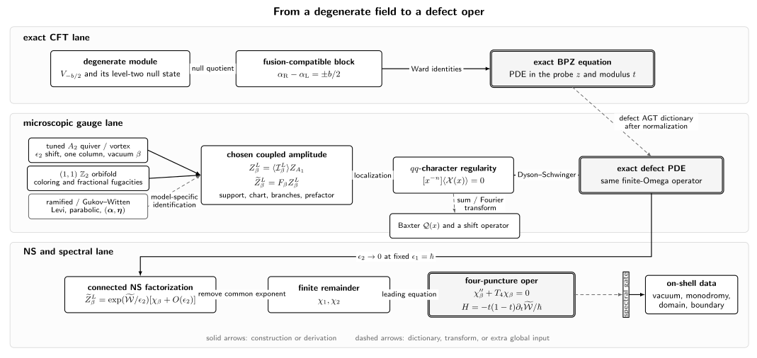
Three gates in the defect route to an ODE. Virasoro degeneracy gives an exact BPZ equation. A chosen vortex, orbifold, or ramified construction contributes the missing microscopic data; in the tuned $A_2$-quiver realization of an $A_1$ bulk theory, qq-character regularity makes its normalized partition function satisfy the same finite-Omega operator. Only the normalized NS remainder is an oper wavefunction, and an additional global condition is still required for a spectrum.

A surface defect needs a passport

Near a codimension-two support $D$, choose polar coordinates $(r,\vartheta)$ in the normal plane. A Gukov–Witten-type singularity begins with

$$A \sim \boldsymbol\alpha\,\dd\vartheta+cdots,$$

where the stabilizer of $\boldsymbol\alpha$ is a Levi subgroup $L$. Magnetic or monopole sectors $\boldsymbol m$ can be weighted by a two-dimensional theta parameter $\boldsymbol\eta$. Schematically, the ramified instanton sum is

$$Z_{\mathrm{ram}} = \sum_{k,\boldsymbol m} t^k \exp \left( \ii\boldsymbol\eta\mathbin{\cdot}\boldsymbol m \right) \int_{\mathcal M_{k,\boldsymbol m}}^{\mathrm{equiv}}1.$$

For $SU(N)$, a composition

$$N=n_1+\cdots+n_M$$

gives $L=S[U(n_1)\times\cdots\times U(n_M)]$. The ordering of the $n_I$ can retain parabolic information not visible in the unordered partition. Thus even the Levi label is not always a complete passport.

The realizations most useful for this chapter compare as follows:

Realization	Microscopic input	Extra variable	Localized object	CFT/ODE role
Ramified or Gukov–Witten	Singular holonomy, Levi/parabolic type, $(\boldsymbol\alpha,\boldsymbol\eta)$, and monopole sectors	A defect coupling or ramified fugacity	Integral over $\mathcal M_{k,\boldsymbol m}$	General framework; not always one Virasoro degenerate field
Orbifold or chain-saw	$\mathbb C_{\epsilon_1}\times(\mathbb C_{\epsilon_2^{\mathrm{orb}}}/\mathbb Z_p)$, a coloring, and fractional couplings	Ratios of fractional fugacities	Colored Young-diagram or parabolic-sheaf sum	In the $A_1$, $(1,1)$ case, another chart of the BPZ solution space
Vortex or quiver	An auxiliary quiver node, equivariant Higgsing, support plane, and vacuum $\beta$	A two-dimensional FI/Kähler fugacity	A one-column sum coupled to the bulk instantons	Realizes the light degenerate insertion in the worked convention
NS oper remainder	A chosen normalized defect function and $\epsilon_2\to0$ path	The same $z$ after its chart is fixed	The $O(\epsilon_2^0)$ factor $\chi_\beta$	Oper wavefunction, not a new microscopic defect

For the orbifold construction used below,

$$\mathbb C_{\epsilon_1} \times \left( \mathbb C_{\epsilon_2^{\mathrm{orb}}}/\mathbb Z_p \right), \qquad (w_1,w_2) \longmapsto (w_1,\zeta w_2),$$

so the defect is supported on the $\epsilon_1$-plane $w_2=0$ and $\epsilon_2^{\mathrm{orb}}$ is the cover-plane normal weight. Under $\widetilde w_2=w_2^p$, the quotient maps to a bulk plane with $\widetilde\epsilon_2=p\epsilon_2^{\mathrm{orb}}$. Every later finite-Omega formula renames this effective bulk weight $\widetilde\epsilon_2$ as the book’s $\epsilon_2$. A coloring

$$c:\{1,\ldots,N\}\longrightarrow\mathbb Z_p$$

specifies the projection of the gauge framing. Its fractional couplings may be written

$$\begin{aligned} \mathfrak q_\omega &= \frac{z_{\omega+1}}{z_\omega}, && 0\leq\omega\leq p-2, \\ \mathfrak q_{p-1} &= t\frac{z_0}{z_{p-1}}, && \prod_{\omega=0}^{p-1}\mathfrak q_\omega=t. \end{aligned}$$

The product is the bulk fugacity; the independent ratios are defect Kähler data. For $N=p=2$, a bijective coloring gives the full $(1,1)$ defect used later.

The reciprocal convention changes the Kac label

AGGTV uses $\epsilon_1=b_{\mathrm{src}}\hbar$ and $\epsilon_2=\hbar/b_{\mathrm{src}}$, hence $b_{\mathrm{src}}=b^{-1}$ here. Its $\Phi_{2,1}=V_{-b_{\mathrm{src}}/2}$ is the book’s dual field $V_{-1/(2b)}$. Exchanging the two Omega planes exchanges $b\leftrightarrow b^{-1}$, row and column restrictions, and the two Kac labels. This page keeps the defect on the $\epsilon_1$-plane, uses the $\epsilon_2$ tuning below, and matches the book’s light $V_{-b/2}$ presentation.

One-column Higgsing manufactures the missing coordinate

Start with a $U(N)$ $A_2$ linear quiver. Denote the two external flavor arrays by $\boldsymbol A_0$ and $\boldsymbol A_3$, the auxiliary-node Coulomb parameters by $\boldsymbol A_1$, and the surviving bulk-node parameters by $\boldsymbol A_2$. Choose $\beta\in\{1,\ldots,N\}$ and impose

$$A_{1,\alpha} = A_{0,\alpha} - \epsilon_2\delta_{\alpha\beta}.$$

Zeros in the bifundamental fixed-point weight eliminate every Young diagram at the auxiliary node except

$$\boldsymbol Y^{(1)} = \left( \varnothing,\ldots, \underbrace{(1^k)}_{\beta\text{th color}}, \ldots,\varnothing \right), \qquad k\geq0.$$

This is more than a convenient truncation. The auxiliary instanton number becomes a vortex number on the $\epsilon_1$-plane. With $\mathfrak q_1=z^{-1}$ for the auxiliary node and $\mathfrak q_2=t$ for the bulk node, define

$$\begin{aligned} Z_\beta^L(z,t) :={}& Z_{A_2} \left( \boldsymbol A_0; \boldsymbol A_0-\epsilon_2\boldsymbol e_\beta; \boldsymbol A_2; \boldsymbol A_3 \right. \\ &\left. \mathrel{\Big|} \epsilon_1,\epsilon_2; \mathfrak q_1=z^{-1},\mathfrak q_2=t \right). \end{aligned}$$

Localization reorganizes it as an observable in the one-node bulk theory,

$$Z_\beta^L = \left\langle \mathcal I_\beta^L(z) \right\rangle_{A_1} Z_{A_1}.$$

In the zero-bulk-instanton sector, $\mathcal I_\beta^L$ is the vortex partition function of a two-dimensional GLSM whose target is the total space of

$$\operatorname{Hom} \left( \mathcal O(-1),\mathbb C^N \right) \longrightarrow \mathbb P^{N-1},$$

with Kähler fugacity $z^{-1}$. Nonzero bulk diagrams replace the classical characteristic polynomial in the vortex sum by the bulk $Y$-observable. This coupling is the microscopic content absent from a bulk Nekrasov function.

The zero-bulk-instanton sector is an instructive checksum. Define

$$\mathcal A_2(x) = \prod_{\gamma=1}^{N} \left(x-A_{2,\gamma}\right), \qquad \mathcal P_0(x) = \prod_{\gamma=1}^{N} \left(x-A_{0,\gamma}\right).$$

Then the one-column observable reduces to

$$\mathcal I_{\beta,0}^{L}(z) = \sum_{k=0}^{\infty} z^{-k} \prod_{\ell=1}^{k} \frac{ \mathcal A_2(A_{0,\beta}+\ell\epsilon_1) }{ \mathcal P_0(A_{0,\beta}+\ell\epsilon_1) }.$$

Pulling out powers of $\epsilon_1$ turns this into

$$\begin{aligned} \mathcal I_{\beta,0}^{L}(z) ={}& {}_N F_{N-1} \left( \begin{matrix} 1+\dfrac{A_{0,\beta}-A_{2,1}}{\epsilon_1}, \ldots, 1+\dfrac{A_{0,\beta}-A_{2,N}}{\epsilon_1} \\ \left( 1+\dfrac{A_{0,\beta}-A_{0,\gamma}}{\epsilon_1} \right)_{\gamma\neq\beta} \end{matrix} ;\, z^{-1} \right). \end{aligned}$$

For rank two this is a Gauss function. The choice of $\beta$ selects which denominator parameter is replaced by the factorial $k!$, making the vacuum label visible already before the four-dimensional instanton corrections are restored.

For $N=2$, the choices $\beta=1,2$ are the two massive vacua of the defect GLSM. They will furnish two solutions of one common second-order operator. Calling them the two degenerate fusion channels is justified only after the AGT mass map, scalar prefactor, and local exponents have been matched.

qq-character regularity closes the finite-Omega equation

A $qq$-character $\mathcal X(x)$ is assembled from $Y$-observables so that its normalized expectation value is regular in the spectral variable:

$$\left\langle \mathcal X(x) \right\rangle = T(x), \qquad T(x)\ \text{polynomial}.$$

Consequently every negative Laurent coefficient vanishes,

$$\left[x^{-n}\right] \left\langle \mathcal X(x) \right\rangle =0, \qquad n\geq1.$$

These are the nonperturbative Dyson–Schwinger equations. Under the one-column restriction, moments of the column height become derivatives with respect to $z$, while the bulk instanton number becomes $t\partial_t$. Concretely, $z\partial_z(z^{-k})=-kz^{-k}$, so the first two column moments are represented by $z\partial_z$ and $(z\partial_z)^2$. For $N=2$, an appropriate negative Laurent coefficient therefore closes on $Z_\beta^L$ and gives a second-order PDE. Without the one-column restriction, the same coefficient contains independent shape observables and need not close on one scalar function.

The raw localization sum must first be conjugated by an explicit multivalued prefactor. Write

$$\widetilde Z_\beta^L = F_\beta(z,t)Z_\beta^L.$$

For the moment use the source’s $U(2)$ variables, set $\epsilon_\Sigma=\epsilon_1+\epsilon_2$, and define $\bar A_i=(A_{i,1}+A_{i,2})/2$. The four dimensionless weights are

$$\begin{aligned} \Delta_0 &= \frac{ \epsilon_\Sigma^2-(A_{3,1}-A_{3,2})^2 }{4\epsilon_1\epsilon_2}, \\ \Delta_t &= -\frac{ (\bar A_2-\bar A_3) (\bar A_2-\bar A_3+\epsilon_\Sigma) }{\epsilon_1\epsilon_2}, \\ \Delta_1 &= -\frac{ (2\bar A_0-2\bar A_2+2\epsilon_1+\epsilon_2) (2\bar A_0-2\bar A_2-\epsilon_2) }{4\epsilon_1\epsilon_2}, \\ \Delta_\infty &= \frac{ \epsilon_\Sigma^2-(A_{0,1}-A_{0,2})^2 }{4\epsilon_1\epsilon_2}. \end{aligned}$$

The degenerate weight is

$$\Delta_{\mathrm d} = -\frac12- \frac{3\epsilon_2}{4\epsilon_1}.$$

In this normalization, the exact operator is

$$\begin{aligned} 0 ={}& \bigg[ \epsilon_1^2\partial_z^2 - \epsilon_1\epsilon_2 \left( \frac1z+ \frac1{z-1} \right) \partial_z \\ &\quad+ \epsilon_1\epsilon_2 \frac{ t(t-1) }{ z(z-1)(z-t) } \partial_t \\ &\quad+ \epsilon_1\epsilon_2 U_\Omega(z,t) \bigg] \widetilde Z_\beta^L, \end{aligned}$$

where

$$\begin{aligned} U_\Omega(z,t) ={}& \frac{\Delta_0}{z^2} + \frac{\Delta_t}{(z-t)^2} + \frac{\Delta_1}{(z-1)^2} \\ &+ \frac{ \Delta_\infty- \Delta_0- \Delta_t- \Delta_1- \Delta_{\mathrm d} }{z(z-1)}. \end{aligned}$$

Divide by $\epsilon_1\epsilon_2$ and use $b^2=\epsilon_2/\epsilon_1$. The result is exactly the five-point BPZ operator printed on the preceding page after the source modulus $\mathfrak q$ is renamed $t$. In particular,

$$-\Delta_{\mathrm d} = \frac{2\epsilon_\Sigma+\epsilon_2}{4\epsilon_1}$$

is the small constant that makes the simple-pole coefficient agree. This equality is a stringent convention check: a plane exchange or a missing prefactor changes the printed operator.

The CFT null-state derivation and the gauge qq-character derivation are separately exact in their stated categories. The former is an identity inside a fusion-compatible Virasoro block; the latter is an all-instanton formal-localization identity for the tuned quiver. The defect extension of AGT identifies their normalized solutions. It should not be promoted from this model-specific result to the statement that every ramified defect is a Virasoro degenerate insertion.

The exact conjugating prefactor

The two local exponents selected by the defect vacuum are

$$\begin{aligned} r_{L,1} &= \frac{ -A_{0,1}+A_{0,2}+\epsilon_\Sigma+\epsilon_2 }{2\epsilon_1}, \\ r_{L,2} &= \frac{ A_{0,1}-A_{0,2}+\epsilon_\Sigma+\epsilon_2 }{2\epsilon_1}. \end{aligned}$$

Up to a $z$- and $t$-independent constant, Jeong–Nekrasov’s left-chart normalization is

$$\begin{aligned} F_\beta(z,t) ={}& \left(-\frac1z\right)^{-r_{L,\beta}} t^{\sigma_t} \left(1-\frac1z\right)^{\sigma_1} \\ &\times \left(1-\frac tz\right)^{\sigma_{tz}} (1-t)^{\sigma_{\mathcal H}}, \end{aligned}$$

with

$$\begin{aligned} \sigma_t &= -\Delta_t-\Delta_0 + \frac{ \epsilon_\Sigma^2-(A_{2,1}-A_{2,2})^2 }{4\epsilon_1\epsilon_2}, \\ \sigma_1 &= \frac{ 2\bar A_0-2\bar A_2+2\epsilon_1+\epsilon_2 }{2\epsilon_1}, \\ \sigma_{tz} &= \frac{ \bar A_2-\bar A_3+\epsilon_\Sigma }{\epsilon_1}, \\ \sigma_{\mathcal H} &= \frac{ 2(\bar A_2-\bar A_3+\epsilon_\Sigma) (2\bar A_0-2\bar A_2-\epsilon_2) }{\epsilon_1\epsilon_2}. \end{aligned}$$

All powers require logarithm branches. If $\mathcal D_{\mathrm{raw}}Z_\beta^L=0$, then the operator on the normalized function is

$$\mathcal D_{\mathrm{BPZ}} = F_\beta \mathcal D_{\mathrm{raw}} F_\beta^{-1}.$$

The factor is therefore part of the dictionary, not cosmetic display formatting. Page 5 translates these source variables into centered masses and Liouville momenta.

The equation acts on the full constrained coupled amplitude $Z_\beta^L=\langle\mathcal I_\beta^L\rangle Z_{A_1}$ after multiplication by $F_\beta$. It does not act unchanged on the normalized expectation $\langle\mathcal I_\beta^L\rangle$ alone. Here full coupled means that the bulk $A_1$ instanton factor has not been divided away; it does not mean that a coupling-independent four-dimensional one-loop factor has already been restored. Indeed, if a bulk factor $g(t)$ is removed, then

$$g^{-1} \partial_t g = \partial_t+\partial_t\Log g,$$

and the last term shifts the accessory coefficient. This elementary conjugation is the gauge-theory version of the distinction between full and unit-leading conformal blocks.

To reconnect the source variables with the regular AGT passport, write any external weight as

$$\Delta_f = \frac{ \epsilon_\Sigma^2-4p_f^2 }{4\epsilon_1\epsilon_2}.$$

In that passport,

$$\begin{array}{c|c} \text{puncture datum} & \text{printed localization masses} \\ \hline 2p_\infty & \mu_1-\mu_2 \\ 2p_1 & \mu_1+\mu_2-\epsilon_\Sigma \\ 2p_t & \mu_3+\mu_4-\epsilon_\Sigma \\ 2p_0 & \mu_3-\mu_4 \end{array}$$

and the internal weight uses

$$\Delta_I = \frac{ \epsilon_\Sigma^2-4a_{\mathrm C}^2 }{4\epsilon_1\epsilon_2}.$$

The source’s prefactor then contains the recognizable channel power $t^{\Delta_I-\Delta_t-\Delta_0}$. Its remaining powers depend on the chosen $U(2)$ lift and bulk Heisenberg factor. They must be translated together; the last exponent in $F_\beta$ should not be renamed the Page 2 Heisenberg exponent in isolation.

The two vacua become the two fusion branches

The operator above is independent of $\beta$. At generic parameters its two left-chart solutions have leading powers

$$\widetilde Z_\beta^L \sim z^{r_{L,\beta}} t^{\Delta_I-\Delta_t-\Delta_0} \left( 1+O(z^{-1},t) \right).$$

Using $A_{0,1}-A_{0,2}=2p_\infty$, the two values of $r_{L,\beta}$ are precisely the powers associated, after the scalar prefactor is included, with the two adjacent momenta

$$\alpha_\infty-\frac b2, \qquad \alpha_\infty+\frac b2.$$

Equivalently, if $s=\pm1$ labels the sign, the CFT indicial power can be written

$$r_s = \Delta_\infty - \Delta_{\mathrm d} - \Delta \left( \alpha_\infty+s\frac b2 \right).$$

Thus the chain of identifications is

$$\text{color }\beta \longleftrightarrow \text{massive defect vacuum} \longleftrightarrow \text{local exponent} \longleftrightarrow \text{fusion sign}.$$

It is not a chain of Coulomb-Weyl branches. A Coulomb reflection acts on the bulk internal momentum, whereas $\beta$ selects a vacuum of the two-dimensional defect. At a resonance where the two indicial roots differ by an integer, the operator remains valid but the two unit-leading power series may need a logarithmic or limiting basis.

Vortex and orbifold sums are different analytic charts

The three natural localization expansions for the rank-two $A_1$ example occupy different annuli:

Basis of defect functions	Natural expansion variables	Initial domain
Left quiver/vortex $\widetilde{\boldsymbol Z}^{L}$	$(z^{-1},t)$	$0<
$(1,1)$ $\mathbb Z_2$ orbifold $\widetilde{\boldsymbol Z}^{\mathbb Z_2}$	$(z,t/z)$	$0<
Right quiver/vortex $\widetilde{\boldsymbol Z}^{R}$	$(t,z/t)$	$0<

No two rows are equal merely by comparing their first few terms in their original variables. Barnes-type contour representations continue the quiver sums into the middle annulus. There, uniqueness of the generic second-order equation and matching indicial data give the exact rank-two identity

$$\widetilde{\boldsymbol Z}^{L\to M} (\boldsymbol A_2) = \boldsymbol S \widetilde{\boldsymbol Z}^{R\to M} (\boldsymbol A_2) = \widetilde{\boldsymbol Z}^{\mathbb Z_2} (\boldsymbol A_2),$$

where

$$S_{\alpha\beta} = \exp \left( \epsilon_2\partial_{A_{2,\alpha}} \right) \delta_{\alpha\beta}.$$

The equality concerns normalized protected partition functions after analytic continuation, the cover-to-bulk rescaling $\widetilde\epsilon_2=p\epsilon_2^{\mathrm{orb}}$, and a Coulomb shift. It does not prove that the three ultraviolet definitions are literally identical field theories.

The rank-two uniqueness argument must not be extrapolated blindly. At rank three the finite-Omega differential system also contains a chiral observable not fixed by that single equation. In Jeong–Nekrasov the three NS oper solutions match, while equality of the full generic finite-Omega functions is proposed and checked only to low orders. Likewise, a general Levi defect can lead to affine or $W$-algebra Ward systems rather than the scalar Virasoro equation on this page.

The NS remainder is the oper wavefunction

Take the book’s NS direction

$$\epsilon_1=\hbar\ \text{fixed}, \qquad \epsilon_2\longrightarrow0, \qquad b\longrightarrow0.$$

For the already conjugated defect amplitude, assume the connected asymptotic expansion

$$\widetilde Z_\beta^L (\boldsymbol A_2,z,t) = \exp \left[ \frac{ \widetilde{\mathcal W}(\boldsymbol A_2,t) }{\epsilon_2} \right] \left[ \chi_\beta(\boldsymbol A_2,z,t) +O(\epsilon_2) \right].$$

The singular exponent is independent of the local vacuum $\beta$ and of $z$ in this chart. The defect observable contributes the finite remainder $\chi_\beta$. Define

$$\delta_f := \lim_{\epsilon_2\to0} \frac{\epsilon_2}{\hbar} \Delta_f = \frac{1-\theta_f^2}{4},$$

where $\theta_f=2p_f/\hbar$ is held fixed on the centered-mass NS path. The first-derivative term and the derivative $\partial_t\chi_\beta$ are subleading. The leading equation is

$$\left[ \partial_z^2 + T_4(z;t) \right] \chi_\beta(z,t) =0,$$

with

$$\begin{aligned} T_4(z;t) ={}& \frac{\delta_0}{z^2} + \frac{\delta_t}{(z-t)^2} + \frac{\delta_1}{(z-1)^2} \\ &- \frac{ \delta_0+\delta_t+\delta_1-\delta_\infty }{z(z-1)} + \frac{H}{z(z-1)(z-t)}. \end{aligned}$$

The accessory coefficient is

$$H = -\frac{t(1-t)}{\hbar} \partial_t\widetilde{\mathcal W} = t(t-1)c_t^{\mathrm{op}},$$

where

$$c_t^{\mathrm{op}} = \frac1\hbar \partial_t\widetilde{\mathcal W}.$$

This sign agrees with the moving-pole residue convention on Page 2. The equality also shows why a $t$-dependent factor cannot be dropped: it changes $\widetilde{\mathcal W}$ and hence $H$. The particular Jeong–Nekrasov derivation omits a $t$-independent one-loop contribution from $\widetilde{\mathcal W}$. That omission does not change the displayed $t$ derivative, but it matters for the full generating function, connection normalizations, and monodromy data.

At generic Coulomb modulus the oper is off shell. Its coefficient $H$ is a coordinate on the variety of opers, not yet a discrete eigenvalue. An on-shell spectrum requires an additional Lagrangian-brane intersection, Bethe-vacuum condition, monodromy constraint, or operator domain. The quantum-curve passport and the nonperturbative-completion page explain that final gate.

Differential and difference curves use different polarizations

The object just derived is differential in the defect coordinate $z$: at finite Omega it is a BPZ PDE in $(z,t)$, and in the NS limit it is an oper ODE in $z$. At finite Omega, the same localization construction represents the defect amplitude as an exact weighted sum of $\mathcal Q$-observables depending on an additive spectral coordinate $x$. After NS factorization, those observables reduce to Baxter $\mathcal Q$-functions, and the oper equation can be interpreted as a Fourier transform of a relation such as

$$\mathcal T(x)\mathcal Q(x) = A(x)\mathcal Q(x+\hbar) + D(x)\mathcal Q(x-\hbar).$$

This relates solution spaces after the transform; it does not turn $\partial_z$ into a finite difference in the same variable. A quantization passport must therefore state:

Question	Differential presentation	Difference presentation
Coordinate	Defect FI/position variable $z$	Additive spectral variable $x$
Operator	BPZ PDE, then oper ODE	Baxter $\mathcal T\mathcal Q$ shift operator after NS reduction
Finite-Omega statement	Exact for the tuned protected amplitude	Exact qq-character and $\mathcal Q$-observable identities; not yet the ordinary NS Baxter function
Bridge	Integral, sum, or Fourier transform plus normalization	Inverse transform and analytic data

Higher-rank defects can give higher-order scalar operators or KZ-like systems. The phrase quantum curve should name the declared operator and polarization, not erase this distinction.

Bulk AGT does not choose the defect

The ordinary four-point AGT block fixes none of the following:

• the new coordinate $z$ or a two-dimensional FI/Kähler parameter;
• which Omega plane supports the defect and therefore which Kac label is light in the book convention;
• a Gukov–Witten Levi/parabolic type, orbifold order, coloring, or ramified monopole sector;
• the Higgsing path and the defect vacuum $\beta$;
• the raw localization measure, multiplicative prefactor, and logarithm branches;
• the defect $qq$-character or nonperturbative Dyson–Schwinger identity;
• the convergence annulus and continuation path;
• an NS factorization, oper lift, or spectral boundary condition.

Those entries form the defect passport. For the worked construction, the compact form is:

Key	Forward datum	Reverse audit
Bulk frame	$A_1$ four-puncture theory in the $0t$ channel	Recover punctures $(0,t,1,\infty)$ and the bulk fugacity $t$
Microscopic defect	Tuned $A_2$ quiver, or the matched $(1,1)$ $\mathbb Z_2$ orbifold	Recover the Higgsing equation, or the orbifold order, coloring, and cover-to-bulk weight rescaling
Support	$\epsilon_1$-plane; $\epsilon_2$ is normal	Check that column contents advance by $\epsilon_1$ and the tuning shifts by $\epsilon_2$
Defect variable	$\mathfrak q_1=z^{-1}$ in the left chart	Recover the declared annulus before expanding or continuing
Discrete label	$\beta=1,2$	Recover the colored column, GLSM vacuum, local exponent, and fusion sign
Raw function	$Z_\beta^L=\langle\mathcal I_\beta^L\rangle Z_{A_1}$	Do not silently replace it by $\langle\mathcal I_\beta^L\rangle$
Normalization	The complete $F_\beta(z,t)$ and logarithm branches	Conjugate the raw operator back and reproduce every local power
Ward identity	Polynomial $qq$-character expectation	Verify that the relevant negative Laurent coefficient vanishes
Finite-Omega object	BPZ PDE in $(z,t)$	Recover $b^2=\epsilon_2/\epsilon_1$ and $\Delta_{\mathrm d}$
NS object	$\widetilde{\mathcal W}$ and the remainder $\chi_\beta$	Restore the common exponent and check $H=t(t-1)\partial_t\widetilde{\mathcal W}/\hbar$
Global completion	Not supplied on this page	Specify continuation, monodromy basis, vacuum equation, domain, and boundary condition

The forward entries are exact formal-localization data for generic equivariant parameters away from poles of the fixed-point weights. The reverse local basis assumes nonresonant exponent differences; at resonance the operator survives but the basis must be obtained by a logarithmic or limiting prescription. The quiver/orbifold equality uses the middle annulus and the Coulomb shift displayed above. AGGTV supplies the proposal and physical evidence for the CFT/defect bridge; Nekrasov’s and Jeong–Nekrasov’s $qq$-character derivations supply the model-specific finite-Omega identity; Kanno–Tachikawa supplies the Levi/parabolic warning.

Once these entries are declared, the worked $A_1$ construction supplies a reversible chain

$$\begin{gathered} \text{one-column defect localization} \xrightarrow{\ qq\text{-character}\ } \text{finite-Omega BPZ PDE}, \\ \text{finite-Omega BPZ PDE} \xrightarrow{\ \epsilon_2\to0\ } \text{Heun oper plus }H, \\ \text{Heun oper plus }H \xrightarrow{\ \text{global condition}\ } \text{possible on-shell spectrum}. \end{gathered}$$

Only the first two arrows are established on this page. The last is a separate spectral problem.

Common pitfalls

Using a degenerate numerical weight without the fusion rule. The null state decouples in the degenerate quotient and compatible sewing channel. An arbitrary analytic continuation of a generic block need not obey the two-channel BPZ system.

Calling every surface defect a vortex. A singular ramified defect, an orbifold/chain-saw construction, and a Higgsed vortex GLSM are different ultraviolet descriptions. Compare protected functions only after their Levi/coloring, support, parameters, and continuation have been matched.

Applying the BPZ operator to the wrong normalization. The displayed equation annihilates $F_\beta Z_\beta^L$, not the raw sum and not $Z_\beta^L/Z_{A_1}$ with the same coefficients. A $t$-dependent division shifts the accessory term.

Calling the finite-Omega equation a Heun ODE. Its $t$ derivative is nonzero. The Heun oper arises only after the connected NS asymptotic turns that derivative into $\partial_t\widetilde{\mathcal W}$.

Equating the oper accessory with a spectrum. Generic Coulomb data give an off-shell oper. Quantization requires global boundary, monodromy, brane, or Bethe-vacuum data.

Exercises

1. Translate the plane and Kac label

The book uses $b^2=\epsilon_2/\epsilon_1$ and keeps the defect on the $\epsilon_1$-plane. Explain why an $\epsilon_2$ Higgsing shift and a single column advancing in steps of $\epsilon_1$ correspond to the book’s $V_{-b/2}$. Translate this field into AGGTV’s reciprocal $b_{\mathrm{src}}$ convention.

Solution

The column contents advance along the tangent equivariant direction $\epsilon_1$, while the tuning uses the normal weight $\epsilon_2$. With $b^2=\epsilon_2/\epsilon_1$, this is the light book field $V_{-b/2}$, conventionally the book’s $(2,1)$ label.

AGGTV has $b_{\mathrm{src}}^2=\epsilon_1/\epsilon_2=b^{-2}$, so

$$-\frac b2 = -\frac{1}{2b_{\mathrm{src}}}.$$

It is therefore AGGTV’s dual $(1,2)$ field. Exchanging the two planes transposes the row/column restriction and exchanges the two labels.

2. Audit the constant in the finite-Omega operator

Show that the simple-pole coefficient in the Jeong–Nekrasov operator equals the CFT coefficient containing $\Delta_{\mathrm d}$.

Solution

Since $\epsilon_\Sigma=\epsilon_1+\epsilon_2$,

$$\frac{2\epsilon_\Sigma+\epsilon_2}{4\epsilon_1} = \frac12+ \frac{3\epsilon_2}{4\epsilon_1} = -\Delta_{\mathrm d}.$$

Therefore

$$\begin{aligned} &- \left[ -\frac{2\epsilon_\Sigma+\epsilon_2}{4\epsilon_1} +\Delta_0+\Delta_t+\Delta_1-\Delta_\infty \right] \\ &\qquad= \Delta_\infty- \Delta_0- \Delta_t- \Delta_1- \Delta_{\mathrm d}, \end{aligned}$$

which is the BPZ numerator.

3. See the accessory shift under bulk normalization

Let $\mathcal D$ contain $K(z,t)\partial_t$ and suppose $\mathcal D\widetilde Z=0$. Set $\widetilde Z=g(t)\widehat Z$. Find the operator on $\widehat Z$.

Solution

Substitution gives

$$\partial_t\widetilde Z = g \left( \partial_t+\partial_t\Log g \right) \widehat Z.$$

Hence the conjugated operator is

$$g^{-1}\mathcal Dg = \mathcal D + K(z,t)\partial_t\Log g,$$

with the derivative understood to act no further on the last term. The new rational zeroth-order term shifts the moving-pole accessory.

4. Derive the NS accessory sign

Insert $\widetilde Z=\exp(\widetilde{\mathcal W}/\epsilon_2) (\chi+O(\epsilon_2))$ into the finite-Omega equation and derive the coefficient $H$.

Solution

The modulus term contributes at leading order

$$\epsilon_1 \frac{t(t-1)}{z(z-1)(z-t)} \partial_t\widetilde{\mathcal W}.$$

After division by $\epsilon_1^2$ with $\epsilon_1=\hbar$, this is

$$\frac{ t(t-1)\hbar^{-1}\partial_t\widetilde{\mathcal W} }{z(z-1)(z-t)}.$$

Thus

$$H = \frac{t(t-1)}\hbar \partial_t\widetilde{\mathcal W} = -\frac{t(1-t)}\hbar \partial_t\widetilde{\mathcal W}.$$

5. Recover the orbifold annulus

For the $\mathbb Z_2$ defect take fractional couplings $\mathfrak q_0=-z$ and $\mathfrak q_1=-t/z$. Determine the domain in $(z,t)$ when both fractional series converge for $0<|\mathfrak q_0|,|\mathfrak q_1|<1$.

Solution

The two inequalities are

$$|z|<1, \qquad \left|\frac tz\right|<1.$$

Together with nonzero fugacities they give

$$0<|t|<|z|<1,$$

the intermediate annulus between the two quiver charts.

6. Distinguish a vacuum label from a Weyl branch

State what $\beta=1,2$ selects in the tuned quiver and what the bulk Weyl reflection selects. Why can the two operations not be identified?

Solution

The label $\beta$ chooses which auxiliary-node color supports the one column. It is a massive vacuum of the two-dimensional GLSM and fixes a local exponent or degenerate fusion sign. The bulk Weyl reflection sends $a_{\mathrm C}\mapsto-a_{\mathrm C}$ and reflects the internal Liouville momentum. One acts on defect-vacuum data and the other on the bulk tube label; they may be related by additional symmetries in special normalizations but are not the same operation.

7. Diagnose an incomplete defect claim

Someone writes

$$Z_{\mathrm{Nek}}(a,t) = \psi(z).$$

List four independent missing data that already prevent this from being a meaningful equality.

Solution

Any four of the following suffice: a microscopic defect realization; the support plane; the source of $z$ and its chart; a Levi or coloring; the vacuum $\beta$; the raw versus normalized partition function; the conjugating prefactor and logarithm branches; the defect Ward identity; the NS limiting path; and a spectral boundary condition. The bulk function on the left has no $z$ at all, while the right-hand side also pretends that a wavefunction and a spectrum have already been selected.

8. Separate the differential and difference variables

In the NS polarization, suppose a defect amplitude is a transform

$$\chi(z) = \sum_{n\in\mathbb Z} z^n\mathcal Q(x_0+n\hbar).$$

Explain why a Baxter shift equation for $\mathcal Q(x)$ does not imply that the BPZ equation is a finite-difference equation in $z$.

Solution

The shift $x\mapsto x\pm\hbar$ changes the lattice index $n$ under the transform. Multiplication by $z^{\pm1}$ and differentiation such as $z\partial_z$ act on that index in the transformed representation. Thus the transform can intertwine two different operator representations, but it does not identify their coordinates or their printed actions. The Baxter operator is difference in $x$; the BPZ operator remains differential in $z$.

References

• A. A. Belavin, A. M. Polyakov, and A. B. Zamolodchikov, “Infinite Conformal Symmetry in Two-Dimensional Quantum Field Theory”, Nuclear Physics B 241 (1984), 333–380. Null-state decoupling and conformal Ward identities are the exact CFT origin of the BPZ differential equation used here.
• L. F. Alday, D. Gaiotto, S. Gukov, Y. Tachikawa, and H. Verlinde, “Loop and Surface Operators in N=2 Gauge Theory and Liouville Modular Geometry”, Journal of High Energy Physics 01 (2010) 113. Equation (2.6) fixes the reciprocal-$b$ convention; Section 2.2, especially equation (2.12) and footnote 6, gives the null equation and fusion restriction; equations (2.14)–(2.16) give the semiclassical open Seiberg–Witten integral. Sections 3.1 and 3.4 give the singular defect data and ramified instanton grading. The paper presents the general degenerate-insertion/defect correspondence as a proposal supported by physical evidence.
• N. Nekrasov, “BPS/CFT Correspondence V: BPZ and KZ Equations from qq-Characters”, arXiv:1711.11582. Equations (17)–(18) state qq-character polynomiality, equations (25)–(33) derive the BPZ equation and identify the normalized tuned quiver partition function. Equation (44) and the paragraph following it explain the one-column vortex sector. This is the exact formal-localization result used to sharpen the earlier proposal.
• S. Jeong and N. Nekrasov, “Opers, Surface Defects, and Yang–Yang Functional”, Advances in Theoretical and Mathematical Physics 24 (2020), 1789–1916. Sections 2.1–2.2 construct the quiver and orbifold defects. Equations (3.14)–(3.17) fix the conjugating prefactor and finite-Omega operator; equations (3.18)–(3.23) give the NS oper and accessory. Section 4.2 proves the rank-two analytic-continuation identity and states the higher-rank limitation.
• H. Kanno and Y. Tachikawa, “Instanton Counting with a Surface Operator and the Chain-Saw Quiver”, Journal of High Energy Physics 06 (2011) 119. Sections 2.1–2.4 relate Levi/parabolic data, ramified instantons, orbifold sheaves, and the chain-saw fixed-point sum, and show why the ordered composition is finer than the unordered Levi partition.
• S. Jeong, “Splitting of Surface Defect Partition Functions and Integrable Systems”, Nuclear Physics B 938 (2019), 775–806. The paper gives finite-Omega differential defect equations in asymptotically free examples and explains their Fourier-transform relation to Baxter difference equations and their NS integrable-system limits.