Stage C: Instanton Transseries, Large Order, and Ambiguity Cancellation

Page 6 turned two admissible endpoint lines into an exact boundary determinant. When that determinant contains an exponentially small Voros symbol, solving it displaces a perturbative root by an exponentially small amount. Repeating the implicit solution produces an instanton transseries for the spectral parameter.

That formal enlargement is not optional decoration. On a singular Borel ray, the perturbative series has two lateral sums. Their difference is of the same exponential size as a neighboring instanton sector. A physical answer becomes independent of the lateral choice only after the transseries parameter, or more generally the full collection of sector parameters, transforms with the Stokes automorphism.

This page derives that mechanism from the quantization function, relates neighboring sectors to large-order growth, and then explains the double-well selection rule. Complex turning points and genuinely complex spectra are deferred to Page 8.

The central cancellation law

Fix the convention of Page 2

$$\mathcal S_{\theta+} = \mathcal S_{\theta-}\circ\mathfrak S_\theta.$$

Suppose a closed one-parameter transseries family satisfies

$$\mathfrak S_\theta \widehat E(\sigma) = \widehat E(\sigma+\mathsf S).$$

Then its two balanced lateral representatives agree:

$$\begin{aligned} \mathcal S_{\theta+} \widehat E\!\left(\sigma-\frac{\mathsf S}{2}\right) &= \mathcal S_{\theta-} \widehat E\!\left(\sigma+\frac{\mathsf S}{2}\right) \\ &=: \mathcal S_\theta^{\mathrm{med}} \widehat E(\sigma). \end{aligned}$$

This is a formal-analytic identity, not a claim that every problem has a single translating parameter. Reality additionally requires a real spectral problem, the appropriate conjugation law, and a compatible choice of the balanced parameter.

Status ledger

Statement used on this page	Status
Formal implicit expansion of a simple root in an exponential variable	Exact algebra in a suitable formal transseries ring
Existence of a full resurgent energy transseries	Theorem or model result only after the quantization function, action grading, and summability hypotheses are established
Equality of an exact-WKB action and a Euclidean saddle action	Model- and normalization-dependent identification, not terminology
Translation $\sigma\mapsto\sigma+\mathsf S$	Special closed one-parameter Stokes action; a general Stokes map can be nonlinear and multi-parameter
Median identity in terms of half a Stokes automorphism	Exact formal identity when the half-automorphism exists in the completed action filtration
Median sum is real	Conditional on conjugation, boundary data, and a compatible real parameter
Factorial-over-power large order from a companion sector	Consequence of the stated resurgent singularity and dominance assumptions
Perturbative large order determines an absolute instanton amplitude	False without a sector-normalization convention; it determines Stokes-weighted data
One-instanton splitting controls the double-well perturbative ambiguity	False; the same-vacuum perturbative sector first communicates with a neutral two-event sector
Principal value by itself is the full nonperturbative answer	False in general

An exponential in the determinant becomes a transseries variable

Let the lateral exact quantization function be organized near one perturbative branch as

$$\widehat{\mathcal Q} (E,\hbar;q) = \sum_{r\geq0} q^r\widehat{\mathcal Q}_r(E,\hbar),$$

where

$$q(\hbar) := \hbar^\alpha \exp\!\left(-\frac{A}{\hbar}\right) \widehat q(\hbar).$$

Here $A$ is the leading action with $\operatorname{Re}(A/\hbar)>0$, while $\widehat q$ is a normalized formal fluctuation series with nonzero constant term. In exact WKB, $q$ usually comes from a small cycle or path Voros symbol after its classical exponential has been separated. The power $\hbar^\alpha$ records a one-loop or endpoint normalization and must not be discarded.

For the recursion below, $q$ is temporarily an independent formal variable. If $A=A(E)$ is substituted too early, differentiating $\exp[-A(E)/\hbar]$ produces additional $A'(E)/\hbar$ terms. One can instead promote the relevant Voros symbols and logarithmic partners to independent graded variables, perform the implicit recursion, and then restore their declared $E$-dependence. If one works directly with $q(E)$, those derivative terms must be included explicitly.

For example, set $q_0=q(E_0,\hbar)$ and write $E=E_0+q_0e_1+q_0^2e_2+\cdots$. Then the second coefficient becomes

$$\begin{aligned} e_2 = -\frac1{\mathcal Q_0'} \biggl[ &\mathcal Q_2 +e_1 \left( \mathcal Q_1' +\mathcal Q_1\partial_E\log q \right) \\ &+ \frac12\mathcal Q_0''e_1^2 \biggr]_{E=E_0}. \end{aligned}$$

This moving-action term is one reason a higher instanton sector is not merely a power of the first.

Assume that the perturbative equation

$$\widehat{\mathcal Q}_0(E_0,\hbar)=0$$

has a simple formal root:

$$\partial_E\widehat{\mathcal Q}_0(E_0,\hbar) \neq0.$$

Seek a root in the form

$$\widehat E = E_0+qE_1+q^2E_2+\cdots.$$

Taylor expansion gives, with every quantity on the right evaluated at $E=E_0$,

$$E_1 = -\frac{\widehat{\mathcal Q}_1} {\partial_E\widehat{\mathcal Q}_0},$$

and

$$\begin{aligned} E_2 = -\frac1{\partial_E\widehat{\mathcal Q}_0} \biggl[ &\frac12 \partial_E^2\widehat{\mathcal Q}_0\,E_1^2 \\ &+ \partial_E\widehat{\mathcal Q}_1\,E_1 + \widehat{\mathcal Q}_2 \biggr]. \end{aligned}$$

Higher sectors follow recursively. Thus the first instanton coefficient is not appended by hand: it is the response of the perturbative root to the first exponentially small term in the boundary determinant.

The simple-root hypothesis is load bearing. Near a level collision, exceptional point, or threshold, $\partial_E\widehat{\mathcal Q}_0$ can vanish. The correct local scale may then be $q^{1/2}$ or another Puiseux power, and a uniform multiple-root analysis replaces the formulas above.

A closed implicit laboratory

The elementary model

$$\mathcal Q(E,q) = E-E_*+q\ee^{\lambda E}$$

has the exact root

$$E(q) = E_* -\frac1\lambda W\!\left( \lambda q\ee^{\lambda E_*} \right),$$

where $W$ is Lambert’s function. Its first terms are

$$\begin{aligned} E(q) =E_* &-q\ee^{\lambda E_*} \\ &+\lambda q^2\ee^{2\lambda E_*} \\ &-\frac32\lambda^2q^3 \ee^{3\lambda E_*} +O(q^4). \end{aligned}$$

This toy determinant will be audited below. It illustrates the implicit algebra only; its $q$ has not been derived from an ODE and therefore is not, by itself, an exact-WKB theorem.

“Instanton” names three objects that need a dictionary

The same word is often used at three analytic levels.

Object	Definition	Information required
Euclidean instanton	A finite-action saddle of a Euclidean path integral	Action normalization, endpoints or topological sector, fluctuation determinant, zero and quasi-zero modes
Exact-WKB action	A period or relative period on the spectral double cover	Sheet, cycle or path, orientation, regularization, and chamber
Transmonomial	A formal scale such as $\hbar^\alpha\ee^{-A/\hbar}$	Action branch, power, logarithms, sector normalization, and lateral prescription

In a standard one-dimensional polynomial oscillator these descriptions can often be matched. The match still has to be demonstrated: a WKB cycle may give $2S_I$ when the Euclidean convention calls a single crossing $S_I$, and endpoint factors can change the algebraic power of $\hbar$. For complex saddles there may be no real Euclidean trajectory at all.

The invariant content is the exponential scale and the normalized connection data in the chosen problem. A name such as “one instanton” does not fix either.

The general spectral ansatz needs actions, powers, and logarithms

For $r$ independent small actions, a useful formal template is

$$\begin{aligned} \widehat E(\boldsymbol\sigma;\hbar) = \sum_{\boldsymbol n\in\mathbb N^r} &\boldsymbol\sigma^{\boldsymbol n} \exp\!\left( -\frac{\boldsymbol n\mathbin{\cdot}\boldsymbol A}{\hbar} \right) \\ &\times \hbar^{\boldsymbol n\mathbin{\cdot}\boldsymbol\beta} \sum_{p=0}^{P(\boldsymbol n)} (\log\hbar)^p \widehat E_{\boldsymbol n,p}(\hbar). \end{aligned}$$

Each $\widehat E_{\boldsymbol n,p}$ is ordinarily an asymptotic power series. The data in this display have different origins:

• the actions $\boldsymbol A$ come from critical paths, cycles, or saddle differences;
• the powers $\boldsymbol\beta$ come from Gaussian fluctuations, endpoint normalizations, and zero modes;
• logarithms arise when action sectors resonate or quasi-zero-mode integrals collide;
• the allowed multi-indices and parameter powers are restricted by symmetry, topology, and the boundary condition.

Even when only one action $A$ occurs, the transseries need not reduce to $\sum_n\sigma^n\ee^{-nA/\hbar}\widehat E_n$. A symmetric double well has parity information in odd sectors and genuine Stokes freedom in neutral even sectors. A periodic potential adds a Bloch angle. Several equal or commensurate actions can force logarithmic sectors and a nontrivial parameter lattice.

A transseries parameter is not automatically a coupling

The parameters $\boldsymbol\sigma$ label formal solutions of the resurgent completion. Global boundary data, parity, a Bloch multiplier, or a choice of integration contour fixes the physical member of that family. The Stokes phenomenon changes its coordinates; it does not change the underlying exact eigenvalue.

The Stokes automorphism acts on the family, not just one sector

For a minimal one-parameter family, write

$$\widehat E(\sigma;\hbar) = \sum_{n\geq0} \sigma^n \ee^{-nA/\hbar} \widehat E_n(\hbar).$$

Assume the action ray is $\theta=\arg A$ and the family is closed under the corresponding Stokes automorphism. In the simplest normalization,

$$\mathfrak S_\theta \widehat E(\sigma) = \widehat E(\sigma+\mathsf S),$$

where $\mathsf S$ is the normalized Stokes constant. Combining this with the book’s operational convention gives

$$\mathcal S_{\theta+}\widehat E(\sigma) = \mathcal S_{\theta-} \widehat E(\sigma+\mathsf S).$$

To first exponential order, suppose

$$\operatorname{Disc}^{\mathrm{an}}_\theta \widehat E_0 = \mathsf S\, \ee^{-A/\hbar} \mathcal S_{\theta-}\widehat E_1 +O(\ee^{-2A/\hbar}).$$

Then

$$\begin{aligned} \mathcal S_{\theta+} \widehat E(\sigma_+) = \mathcal S_{\theta-}\widehat E_0 &+ (\sigma_++\mathsf S) \ee^{-A/\hbar} \\ &\times \mathcal S_{\theta-}\widehat E_1 +\cdots. \end{aligned}$$

Equality with the lower lateral representative requires

$$\sigma_-=\sigma_++\mathsf S.$$

The jump belongs to the coordinate $\sigma$, while the resummed spectral value is unchanged.

Median summation uses half the full automorphism

The parameter translation makes the balanced choice transparent:

$$\sigma_+ = \sigma-\frac{\mathsf S}{2}, \qquad \sigma_- = \sigma+\frac{\mathsf S}{2}.$$

For a general closed transseries, the invariant definition is

$$\mathcal S_\theta^{\mathrm{med}} := \mathcal S_{\theta+} \circ\mathfrak S_\theta^{-1/2} = \mathcal S_{\theta-} \circ\mathfrak S_\theta^{1/2}.$$

The half-powers are formal exponentials of $\tfrac12\log\mathfrak S_\theta$ in the completed action filtration. This construction keeps all coupled sectors and composite alien operations. It is stronger than taking the arithmetic mean of two numbers or the real part of each sector separately.

If the ODE, contour, and boundary conditions are real, complex conjugation interchanges the two laterals, and the balanced parameter is compatible with that conjugation, the median sum is real. None of these hypotheses follows from the word “median.”

The Euler pole shows cancellation with every sign visible

Return to Page 1’s nonalternating Euler series,

$$\widehat\Phi_0(\hbar) := \sum_{n=0}^{\infty}n!\hbar^{n+1}, \qquad \mathcal B\widehat\Phi_0(\xi) = \frac1{1-\xi}.$$

For $\hbar>0$, the book’s upper-minus-lower convention gives

$$\begin{aligned} \mathcal S_{0+}\widehat\Phi_0 &= \Phi_{\mathrm{PV}} +\pi\ii\ee^{-1/\hbar}, \\ \mathcal S_{0-}\widehat\Phi_0 &= \Phi_{\mathrm{PV}} -\pi\ii\ee^{-1/\hbar}, \end{aligned}$$

where

$$\Phi_{\mathrm{PV}} = \ee^{-1/\hbar} \operatorname{Ei}(1/\hbar).$$

Adjoin the flat solution

$$\widehat\Phi(\sigma) := \widehat\Phi_0+\sigma\ee^{-1/\hbar}.$$

The Stokes translation is $\mathsf S=2\pi\ii$. Therefore

$$\begin{aligned} \mathcal S_{0+} \widehat\Phi(\sigma-\pi\ii) &= \Phi_{\mathrm{PV}} +\sigma\ee^{-1/\hbar}, \\ \mathcal S_{0-} \widehat\Phi(\sigma+\pi\ii) &= \Phi_{\mathrm{PV}} +\sigma\ee^{-1/\hbar}. \end{aligned}$$

For real $\sigma$, the common value is real. The cancellation is not a mysterious disappearance of imaginary parts: the perturbative lateral ambiguity and the jump of the flat-sector coefficient are the same Stokes datum written in two coordinates.

This is an exact linear calibration, not a spectral model. In an oscillator, the neighboring sector has its own divergent fluctuation series, and cancellation continues recursively through higher action grades.

Large order reads the first loops around a neighboring sector

Write the perturbative tail in the shifted convention of Page 1 as

$$\widehat E_0(\hbar) = e_* + \sum_{g\geq0} e_g^{(0)}\hbar^{g+1}.$$

Suppose the nearest relevant resurgent relation on the chosen determination is

$$\operatorname{Disc}^{\mathrm{an}}_\theta \widehat E_0 = \mathsf S_{01} \ee^{-A/\hbar} \hbar^\beta \mathcal S_{\theta-} \widehat E_1(\hbar) +\text{larger actions},$$

with

$$\widehat E_1(\hbar) = \sum_{k\geq0}e_k^{(1)}\hbar^k.$$

Under the required continuation, growth, and dominance assumptions, Cauchy’s coefficient formula deformed onto the cut at $A$ gives

$$\begin{aligned} e_g^{(0)} \sim \frac{\mathsf S_{01}}{2\pi\ii} \sum_{k=0}^{K-1} e_k^{(1)} \frac{ \Gamma(g+1-\beta-k) }{ A^{g+1-\beta-k} }, \end{aligned}$$

up to the retained loop order and contributions from other singularities. The leading term is

$$e_g^{(0)} \sim \frac{\mathsf S_{01}e_0^{(1)}}{2\pi\ii} \frac{\Gamma(g+1-\beta)} {A^{g+1-\beta}}.$$

For the Euler calibration, $A=1$, $\beta=0$, $\mathsf S_{01}=2\pi\ii$, and $e_0^{(1)}=1$. The formula gives $e_g^{(0)}=\Gamma(g+1)=g!$ exactly.

Thus the perturbative coefficients know the action $A$, the exponent $\beta$, and the products $\mathsf S_{01}e_k^{(1)}$. They do not separate a Stokes constant from the arbitrary normalization of $\widehat E_1$.

Useful estimators and their failure modes

If one positive action dominates and the leading amplitude is nonzero,

$$A_g := (g+1-\beta) \frac{e_g^{(0)}}{e_{g+1}^{(0)}} \longrightarrow A.$$

After estimating $A$ and $\beta$,

$$C_g := \frac{ A^{g+1-\beta}e_g^{(0)} }{ \Gamma(g+1-\beta) } \longrightarrow \frac{\mathsf S_{01}e_0^{(1)}}{2\pi\ii}.$$

These limits can be accelerated, but acceleration cannot repair a wrong singularity model. Equal-modulus actions must be summed before taking a ratio. A conjugate pair produces oscillations. A negative action produces alternating signs. A vanishing leading Stokes-weighted coefficient exposes a more distant singularity or a subleading loop.

For several isolated actions the leading expansion is a sum,

$$e_g^{(0)} \sim \sum_j \frac{\mathsf S_{0j}}{2\pi\ii} \sum_{k\geq0} e_k^{(j)} \frac{ \Gamma(g+1-\beta_j-k) }{ A_j^{g+1-\beta_j-k} }.$$

The closest singularity controls the exponential envelope in $g$, not necessarily every coefficient. More distant actions appear as exponentially small corrections such as $(A_1/A_2)^g$ after the nearest contribution is subtracted.

Logarithmic sectors leave logarithms of the order

Because

$$\partial_\beta^p\hbar^\beta = \hbar^\beta(\log\hbar)^p,$$

a companion sector containing $(\log\hbar)^p$ differentiates the factorial-over-power expression with respect to $\beta$. The result contains $\log g$, polygamma functions, and inverse powers of $g$. Fitting a pure gamma law to a resonant logarithmic sector therefore misidentifies both the amplitude and the exponent.

Large order is consequently a stringent audit of a proposed transseries, but not a substitute for its global boundary condition. It cannot fix a transseries parameter that is exponentially invisible to the formal perturbative branch.

A quartic thimble supplies a nontrivial companion series

The Euler pole has a constant companion sector. A zero-dimensional quartic integral gives an exact next step in which both sectors carry nontrivial divergent fluctuations. It is a resurgence calibration, not a Schrödinger spectral problem.

For $g>0$, define the convergent stable integral

$$Z_{\mathrm{st}}(g) := \frac1{\sqrt{2\pi g}} \int_{\mathbb R} \exp\!\left[ -\frac1g \left( \frac{x^2}{2}+\frac{x^4}{24} \right) \right] \dd x.$$

The analytically continued unstable action profile

$$U_-(x) = \frac{x^2}{2}-\frac{x^4}{24}$$

has critical points

$$x_0=0, \qquad x_\pm=\pm\sqrt6,$$

and the common saddle-action difference

$$A = U_-(x_\pm)-U_-(x_0) = \frac32.$$

The real unstable integral diverges. Its perturbative expansion is defined through analytic continuation or lateral thimbles, not by an ordinary real-axis integral.

Introduce the two formal sectors

$$\begin{aligned} \widehat\Phi_0(g) &= \sum_{n\geq0}a_ng^n, \\ \widehat\Phi_1(g) &= \sum_{n\geq0}b_ng^n, \end{aligned}$$

with

$$\begin{aligned} a_n &= \frac{(4n)!} {96^n(2n)!\,n!}, \\ b_n&=(-1)^na_n. \end{aligned}$$

Thus

$$\begin{aligned} \widehat\Phi_0(g) &= 1+\frac g8+\frac{35g^2}{384}+\cdots, \\ \widehat\Phi_1(g) &= 1-\frac g8+\frac{35g^2}{384}-\cdots. \end{aligned}$$

To use the book’s shifted transform, apply it to $g\widehat\Phi_j$. The two Borel germs are

$$\begin{aligned} \mathcal B(g\widehat\Phi_0)(\xi) &= {}_2F_1\!\left( \frac14,\frac34;1;\frac{\xi}{A} \right), \\ \mathcal B(g\widehat\Phi_1)(\xi) &= {}_2F_1\!\left( \frac14,\frac34;1;-\frac{\xi}{A} \right). \end{aligned}$$

On the first cut, for $\xi>A$, their boundary values obey

$$\begin{aligned} & \mathcal B(g\widehat\Phi_0)(\xi+\ii0) - \mathcal B(g\widehat\Phi_0)(\xi-\ii0) \\ &\qquad= \ii\sqrt2\, \mathcal B(g\widehat\Phi_1)(\xi-A). \end{aligned}$$

Laplace transformation therefore gives

$$\operatorname{Disc}_0^{\mathrm{an}} \widehat\Phi_0 = \ii\sqrt2\, \ee^{-A/g} \mathcal S_0\widehat\Phi_1.$$

The companion-sector formula predicts

$$a_n \sim \frac1{\pi\sqrt2} \sum_{k=0}^{K-1} b_k \frac{\Gamma(n-k)} {A^{n-k}}.$$

The first loop corrections are

$$\begin{aligned} a_n \sim \frac{\Gamma(n)} {\pi\sqrt2\,A^n} \biggl[ 1 &-\frac{3}{16(n-1)} \\ &+ \frac{105} {512(n-1)(n-2)} +\cdots \biggr]. \end{aligned}$$

In particular,

$$n\frac{a_n}{a_{n+1}} \longrightarrow \frac32, \qquad \frac{A^na_n}{\Gamma(n)} \longrightarrow \frac1{\pi\sqrt2}.$$

The stable companion has an independent exact evaluation,

$$\begin{aligned} Z_{\mathrm{st}}(g) = \sqrt{\frac{3}{2\pi g}}\, \ee^{3/(4g)} K_{1/4}\!\left(\frac{3}{4g}\right). \end{aligned}$$

It equals the regular positive-ray sum of $\widehat\Phi_1$. For the completed unstable family

$$\widehat Z(\sigma;g) = \widehat\Phi_0(g) +\sigma\ee^{-A/g}\widehat\Phi_1(g),$$

the Stokes constant is $\mathsf S=\ii\sqrt2$. Hence the upper parameter $-\ii/\sqrt2$ and lower parameter $+\ii/\sqrt2$ give the same balanced real value. In this linear example that value is also the arithmetic mean of the two perturbative laterals; that simplification is not the general definition of median summation.

This laboratory separates three independent checks: saddle geometry fixes $A$, the hypergeometric cut fixes $\mathsf S$, and the exact coefficients test the resulting large-order prediction.

The double well separates splitting from ambiguity

Consider a real symmetric double well with weak positive coupling $g$, two degenerate minima, and one-instanton action $S_I>0$. For a level label $N$ and parity $\varepsilon=\pm1$, the model-dependent expansion has the schematic but structurally important form

$$\begin{aligned} \widehat E_{\varepsilon,N}(g) ={}& \sum_{\ell\geq0} e_{N,\ell}^{(0)}g^\ell \\ &+ \sum_{n\geq1} \left[ \mathcal C_N(g)\ee^{-S_I/g} \right]^n \\ &\quad\times \sum_{p=0}^{n-1} \left[ \log\!\left(-\frac{\kappa}{g}\right) \right]^p \sum_{\ell\geq0} e_{\varepsilon,N;n,p,\ell}g^\ell. \end{aligned}$$

The prefactor $\mathcal C_N(g)$, the positive constant $\kappa$, and the coefficient normalizations depend on the potential convention. The maximum logarithmic power $n-1$ is characteristic of the standard multi-instanton interaction analysis; it is not a universal law for every transseries.

Two selection rules prevent a common misreading.

1. A single instanton changes wells. It produces the leading parity splitting

   $$E_{+,N}-E_{-,N} = O(\ee^{-S_I/g}).$$

2. Perturbation theory about one specified well begins and ends in the same vacuum. Its first neutral nonperturbative neighbor is an instanton–anti-instanton sector with action $2S_I$:

   $$\operatorname{Disc} \widehat E_N^{(0)} = O(\ee^{-2S_I/g}).$$

Consequently, the one-instanton splitting need not be the singularity seen by the leading large order of the common perturbative series. The neutral two-event sector is.

An exact lateral double-well calibration

One precise realization uses the normalization

$$\left[ -\frac{\hbar^2}{2}\frac{\dd^2}{\dd x^2} + \frac{x^2(1+x)^2}{2} \right]\psi = E\psi.$$

For energies below the barrier, let

$$t:=\frac{\Pi_A}{2\pi}, \qquad t_D:=-\ii\Pi_B,$$

in the cycle convention of van Spaendonck and Vonk. Their two lateral quantization conditions can be written

$$\begin{aligned} D_\varepsilon^\pm = 1 +\ee^{\pm2\pi\ii t/\hbar} \mp\ii\varepsilon \ee^{-t_D(t;\hbar)/(2\hbar)} =0, \end{aligned}$$

where $\varepsilon=\pm1$ is parity. This kinetic normalization differs from the unit-kinetic convention used elsewhere in the book, so its periods must not be imported without translation.

The perturbative root is

$$t_0=\hbar\left(N+\frac12\right).$$

Set

$$q(t,\hbar) := \ee^{-t_D(t;\hbar)/(2\hbar)}$$

and $t=t_0+\Delta t^\pm$. The exact implicit displacement is

$$\begin{aligned} \Delta t^\pm = \mp\frac{\ii\hbar}{2\pi} \log\!\left[ 1\mp\ii\varepsilon q(t_0+\Delta t^\pm,\hbar) \right]. \end{aligned}$$

Retaining the $t$-dependence of $q$ gives

$$\begin{aligned} \Delta t^\pm ={}& -\varepsilon\frac{\hbar}{2\pi}q \\ &+ \left[ \mp\frac{\ii\hbar}{4\pi} -\frac{\hbar}{8\pi^2} \partial_t t_D \right]q^2 \\ &+ O(q^3), \end{aligned}$$

with $q$ and $\partial_t t_D$ evaluated at $t_0$. The first correction is real and parity dependent. Lateral imaginary ambiguity first appears at $q^2$, while $q^2=\exp(-t_D/\hbar)$ is the neutral action scale seen by perturbative large order. This explicit calculation is the promised counterexample to the slogan that the first spectral splitting must control the perturbative coefficients.

For $g>0$, the logarithm has two lateral values,

$$\log\!\left(-\frac{\kappa}{g}\right)_{\pm} = \log\!\left(\frac{\kappa}{g}\right) \pm\pi\ii.$$

The imaginary ambiguity carried by the neutral two-instanton term cancels the ambiguity in the lateral Borel sum of the perturbative sector. At the next grades, the ambiguity of a one-instanton fluctuation series communicates with three-instanton sectors, the two-instanton series with four-instanton sectors, and so on. The exact quantization condition fixes the coefficients and signs of this cancellation ladder.

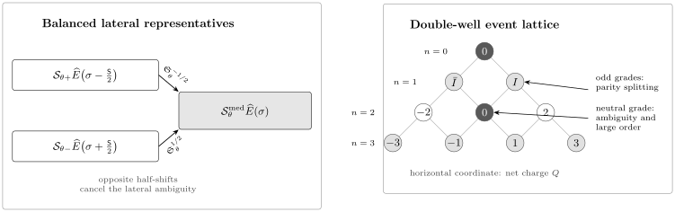
Balanced upper and lower representatives meet after opposite half-Stokes shifts. In the symmetric-double-well event lattice, the vertical coordinate counts instanton events and the horizontal coordinate is the net well-changing charge. Odd sectors control parity splitting, whereas the neutral column communicates with the perturbative vacuum and carries its ambiguity-canceling even sectors. Lattice arrows add an instanton $\mathcal I$ or anti-instanton $\overline{\mathcal I}$; their coefficients are model-dependent Stokes data.

What the triangle does and does not prove

The triangle records action and topological selection rules. It does not compute fluctuation determinants, quasi-zero-mode integrals, Stokes constants, or boundary-condition weights. Nor does it imply that every allowed node is nonzero. Symmetry or a vanishing connection coefficient can remove a sector.

The neutral pair is sometimes called a bion. Depending on the model, its semiclassical representative can involve a correlated saddle rather than a real exact two-event solution. The resurgent statement concerns the normalized sector and its Stokes relation, not the existence of a particular real trajectory.

Exact WKB makes the cancellation a covariance statement

Page 5 supplied the Stokes automorphism of Voros symbols. Page 6 inserted those symbols into a boundary determinant. Combining the two gives the cleanest route to spectral ambiguity cancellation.

For one active saddle class $\delta$, orient $q=\mathcal V_\delta\sim\ee^{-A/\hbar}$ to be small. Page 5’s DDP formula gives, for a relative class $\beta$,

$$\mathcal X_{\beta,+} = \mathcal X_{\beta,-} (1+q_-)^{-\langle\delta,\beta\rangle}.$$

On a continuous logarithmic branch,

$$\begin{aligned} \operatorname{Disc}^{\mathrm{an}} \log\mathcal X_\beta ={}& -\langle\delta,\beta\rangle \log(1+q_-) \\ ={}& -\langle\delta,\beta\rangle \sum_{\ell\geq1} \frac{(-1)^{\ell+1}}{\ell} q_-^\ell. \end{aligned}$$

One primitive active class therefore generates every composite action grade $\ell A$. These coefficients are pieces of the full Stokes automorphism. They are not automatically distinct primitive Euclidean instantons, and raw binomial coefficients should not be relabeled as alien derivatives without taking the logarithm of the automorphism.

Let $\widehat\Delta$ denote the formal determinant in one graph-adapted coordinate system. On a singular direction,

$$\mathcal S_{\theta+}\widehat\Delta = \mathcal S_{\theta-} \left( \mathfrak S_\theta\widehat\Delta \right).$$

The two sides are the same analytic boundary function expressed through the upper and lower lateral connection data. If a simple root is continued consistently, the corresponding energy transseries obeys the induced Stokes map. The root does not acquire a physical ambiguity; its formal coordinates do.

At the formal level, the same statement has a compact implicit chain-rule form. If a homogeneous pointed alien derivation is taken with the moving action lattice locally trivialized, then

$$\begin{aligned} 0 &= \dot\Delta \left[ \widehat{\mathcal Q}(\widehat E,\hbar) \right], \\ \dot\Delta\widehat E &= -\frac{ \left.\dot\Delta_E\widehat{\mathcal Q}\right|_{E=\widehat E} }{ \left.\partial_E\widehat{\mathcal Q}\right|_{E=\widehat E} }. \end{aligned}$$

This identity is conditional on parametric resurgence and the same uniformity in $E$ needed for the analytic implicit problem.

This argument needs four separate ingredients:

1. the DDP or relevant wall-crossing automorphism for every active Voros symbol;
2. a boundary determinant assembled with the same path, sheet, and frame conventions on both sides;
3. a simple root, or an appropriate multiple-root replacement;
4. summability and analytic continuation uniform enough in $E$ to pass the Stokes relation through the implicit solution.

Without the fourth item, formal covariance is not yet an equality of analytic eigenvalues.

Sector normalization changes the reported Stokes constant

Rescale a companion sector by a nonzero constant,

$$\widehat E_1 \longmapsto \lambda\widehat E_1.$$

To keep both the transseries and bridge relation fixed, transform

$$\sigma \longmapsto \frac{\sigma}{\lambda}, \qquad \mathsf S_{01} \longmapsto \frac{\mathsf S_{01}}{\lambda}.$$

Therefore large order determines the invariant product $\mathsf S_{01}e_0^{(1)}$, not either factor separately. A numerical Stokes constant is meaningful only together with the Borel convention, lateral orientation, action branch, and sector normalization.

A practical extraction and cancellation workflow

1. Start from a boundary determinant whose endpoint lines and normalization are already fixed.
2. Choose a chamber and factor every exponentially small Voros symbol into its classical action, algebraic power, and normalized quantum series.
3. Solve the zero-action equation for a simple perturbative root.
4. Expand the determinant recursively in the small transmonomials; allow Puiseux powers or logarithms when the recursion demands them.
5. Derive the Stokes map from the Voros-symbol automorphism and the determinant. Do not infer it only from a desired reality property.
6. Compute many perturbative coefficients and test their large order against the closest permitted companion sectors.
7. Subtract the leading factorial-over-power contribution before fitting a farther action.
8. Fix the physical transseries parameters from parity, Bloch, decay, outgoing, or other global boundary data.
9. Use matched lateral sums or the full median automorphism on a singular ray.
10. Compare against an independent spectral calculation and vary the working precision, truncation, and matching point.

The order matters. A fitted exponential scale is evidence for a Borel singularity, not by itself a proof that a guessed saddle and boundary condition give the correct sector.

Reproducible checks

The companion script instanton-transseries-check.py audits independent representations rather than fitting a formula back to the data that defined it:

• symbolic implicit-root coefficients against the exact Lambert-$W$ laboratory;
• the moving-action term in the exact lateral double-well displacement;
• the signed Euler lateral sums and their median cancellation at high precision;
• quartic saddle geometry, Gaussian moments, an ODE recurrence, and the hypergeometric Borel cut;
• companion-sector large order and the independent Bessel/quadrature evaluation of the stable quartic integral;
• recovery of a farther signed action after exact subtraction of the dominant Borel pole;
• the double-well event lattice rule $|Q|\leq n$ and $Q\equiv n\pmod 2$.

It uses explicit runtime checks rather than Python assert, so optimized mode performs the same audit.

Run it from the project root:

python3 public/code/advanced-ode/instanton-transseries-check.py

These checks verify algebra, signs, and numerical diagnostics. They do not prove resurgence or Borel summability for a new potential.

Common pitfalls

Adding one exponential is not a transseries completion. The fluctuation series around that exponential is generally divergent, its lateral ambiguity couples to higher sectors, and resonance can introduce logarithms. Closure under the relevant Stokes automorphisms is the real test.

A small WKB cycle is not automatically one Euclidean instanton. Orientations, doubled paths, and normalization conventions can change the reported action by a sign or factor of two. Compare the actual exponent, not the label.

The closest positive action need not control every large-order coefficient. Equal-modulus or conjugate singularities can interfere, and selection rules can make the leading Stokes constant vanish. Fit the sum allowed by the geometry.

The Stokes constant depends on a sector basis. Rescaling a companion sector inversely rescales the reported constant. Quote the product tested by large order or state the normalization.

Median is not synonymous with real part. The median operation uses half of the full Stokes automorphism. A termwise principal value can miss coupled sectors and nonlinear parameter maps.

Reality is not universal. It follows for a suitable self-adjoint problem with compatible conjugation. Resonances and non-Hermitian spectra are genuinely complex and are treated on Page 8.

A transseries parameter is fixed globally. Perturbative large order can reveal Stokes-weighted neighboring sectors but not the boundary datum that selects one physical member of the family.

Exercises

1. Derive the first two implicit sectors

Let

$$\mathcal Q(E,q) = \mathcal Q_0(E) +q\mathcal Q_1(E) +q^2\mathcal Q_2(E) +O(q^3),$$

and suppose $\mathcal Q_0(E_0)=0$ with $\mathcal Q_0'(E_0)\neq0$. Derive $E_1$ and $E_2$ for $E=E_0+qE_1+q^2E_2+\cdots$.

Solution

Taylor expansion at $E_0$ gives

$$\begin{aligned} 0 ={}& q\left( \mathcal Q_0'E_1+\mathcal Q_1 \right) \\ &+ q^2 \biggl( \mathcal Q_0'E_2 +\frac12\mathcal Q_0''E_1^2 \\ &\qquad +\mathcal Q_1'E_1 +\mathcal Q_2 \biggr) +O(q^3). \end{aligned}$$

Equating coefficients yields

$$E_1=-\frac{\mathcal Q_1}{\mathcal Q_0'},$$

and

$$E_2 = -\frac{ \tfrac12\mathcal Q_0''E_1^2 +\mathcal Q_1'E_1 +\mathcal Q_2 }{ \mathcal Q_0' }.$$

Every function and derivative on the right is evaluated at $E_0$.

2. Expand the Lambert-W laboratory

Starting from

$$E-E_*+q\ee^{\lambda E}=0,$$

derive the exact Lambert-$W$ solution and its first three nonzero powers of $q$.

Solution

Set $u=\lambda(E_*-E)$. The equation becomes

$$u\ee^u = \lambda q\ee^{\lambda E_*}.$$

Hence

$$E = E_*-\lambda^{-1} W\!\left(\lambda q\ee^{\lambda E_*}\right).$$

Using

$$W(x)=x-x^2+\frac32x^3+O(x^4)$$

gives

$$\begin{aligned} E =E_* &-q\ee^{\lambda E_*} \\ &+\lambda q^2\ee^{2\lambda E_*} \\ &-\frac32\lambda^2q^3 \ee^{3\lambda E_*} +O(q^4). \end{aligned}$$

3. Verify the balanced Euler cancellation

Use the Page 1 lateral sums to show that

$$\mathcal S_{0+}\widehat\Phi(\sigma-\pi\ii) = \mathcal S_{0-}\widehat\Phi(\sigma+\pi\ii)$$

for $\widehat\Phi(\sigma)=\widehat\Phi_0+\sigma\ee^{-1/\hbar}$.

Solution

The upper perturbative sum contains $+\pi\ii\ee^{-1/\hbar}$, while its flat coefficient is $\sigma-\pi\ii$. Their sum is

$$\Phi_{\mathrm{PV}} +\sigma\ee^{-1/\hbar}.$$

The lower perturbative sum contains $-\pi\ii\ee^{-1/\hbar}$, while its flat coefficient is $\sigma+\pi\ii$. It gives the same expression.

4. Extract an action from large order

Assume

$$e_g = C\, \frac{\Gamma(g+1-\beta)} {A^{g+1-\beta}}.$$

Show that

$$(g+1-\beta)\frac{e_g}{e_{g+1}}=A$$

exactly.

Solution

Use $\Gamma(g+2-\beta)=(g+1-\beta)\Gamma(g+1-\beta)$. The constant $C$ and the common power of $A$ cancel, leaving $A$.

5. Reveal a farther Borel singularity

For constants $r_A,r_B$ and $0<|A|<|B|$, let

$$\mathcal B\widehat f(\xi) = \frac{r_A}{A-\xi} +\frac{r_B}{B-\xi}.$$

Find the shifted-Borel coefficients $a_n$ in $\widehat f=\sum_{n\geq1}a_n\hbar^n$. Explain how subtracting the $A$ contribution exposes $B$.

Solution

Expanding each pole at the origin gives

$$\frac{r_A}{A-\xi} = \sum_{n\geq1} \frac{r_A}{A^n}\xi^{n-1},$$

and similarly for $B$. Since the shifted transform has coefficient $a_n/\Gamma(n)$,

$$a_n = \Gamma(n) \left( \frac{r_A}{A^n} +\frac{r_B}{B^n} \right).$$

Subtracting $r_AA^{-n}$ from $a_n/\Gamma(n)$ leaves exactly $r_BB^{-n}$. Ratios of that residual recover $B$, including its phase or sign.

6. Locate the first neutral double-well sector

Let $n_I$ and $n_{\bar I}$ count instantons and anti-instantons. Define

$$n=n_I+n_{\bar I}, \qquad Q=n_I-n_{\bar I}.$$

Show that $|Q|\leq n$ and $Q\equiv n\pmod2$. Which smallest nonzero $n$ returns to the original well?

Solution

Solving for the event numbers gives

$$n_I=\frac{n+Q}{2}, \qquad n_{\bar I}=\frac{n-Q}{2}.$$

They are nonnegative integers precisely when $|Q|\leq n$ and $Q$ has the same parity as $n$. Returning to the original well means $Q=0$, so the smallest nonzero possibility is $n=2$: one instanton and one anti-instanton.

7. Predict the effect of one logarithm on large order

Suppose the discontinuity contains

$$\ee^{-A/\hbar} \hbar^\beta\log\hbar.$$

Use differentiation with respect to $\beta$ to determine the structure of its contribution to $e_g^{(0)}$.

Solution

Differentiate the no-logarithm factor:

$$\partial_\beta \left[ \frac{\Gamma(g+1-\beta)} {A^{g+1-\beta}} \right].$$

Because $\partial_\beta\hbar^\beta =\hbar^\beta\log\hbar$, the result has the required structure. Explicitly,

$$\frac{\Gamma(g+1-\beta)} {A^{g+1-\beta}} \left[ \log A-\psi(g+1-\beta) \right],$$

where $\psi$ is the digamma function. Since $\psi(g+1-\beta)\sim\log g$, the large-order sequence contains a $\log g$ correction.

8. Prove the operator form of the median identity

Starting from

$$\mathcal S_{\theta+} = \mathcal S_{\theta-}\circ\mathfrak S_\theta,$$

show that

$$\mathcal S_{\theta+}\circ\mathfrak S_\theta^{-1/2} = \mathcal S_{\theta-}\circ\mathfrak S_\theta^{1/2}.$$

Solution

Compose the defining relation on the right with $\mathfrak S_\theta^{-1/2}$:

$$\begin{aligned} \mathcal S_{\theta+} \circ\mathfrak S_\theta^{-1/2} &= \mathcal S_{\theta-} \circ\mathfrak S_\theta \circ\mathfrak S_\theta^{-1/2} \\ &= \mathcal S_{\theta-} \circ\mathfrak S_\theta^{1/2}. \end{aligned}$$

The action filtration makes the formal half-power well defined whenever $\log\mathfrak S_\theta$ is.

9. Recover the quartic action from coefficients

Starting from

$$a_n = \frac{(4n)!} {96^n(2n)!\,n!},$$

derive a first-order recurrence and use it to prove $n a_n/a_{n+1}\to3/2$.

Solution

Taking the ratio and canceling adjacent factors gives

$$\frac{a_{n+1}}{a_n} = \frac{(4n+1)(4n+3)} {24(n+1)}.$$

Therefore

$$n\frac{a_n}{a_{n+1}} = \frac{24n(n+1)} {(4n+1)(4n+3)} \longrightarrow \frac{24}{16} = \frac32.$$

The recovered value agrees with the independently computed saddle-action difference.

10. Expand the lateral double-well root

Starting from

$$\Delta t^\pm = \mp\frac{\ii\hbar}{2\pi} \log\!\left[ 1\mp\ii\varepsilon q(t_0+\Delta t^\pm,\hbar) \right],$$

use

$$\partial_t\log q = -\frac{\partial_t t_D}{2\hbar}$$

to derive the terms through $q^2$. Identify the first parity-dependent and the first lateral-ambiguous terms.

Solution

Write

$$q(t_0+\Delta t) = q \left(\partial_t\log q\right)q\,\Delta t +O(q^3).$$

The coefficient of $q$ first gives

$$\Delta t_1 = -\varepsilon\frac{\hbar}{2\pi}q.$$

Substitute this result back into the shifted $q$ and expand the logarithm. The result is

$$\begin{aligned} \Delta t^\pm ={}& -\varepsilon\frac{\hbar}{2\pi}q \\ &+ \left[ \mp\frac{\ii\hbar}{4\pi} -\frac{\hbar}{8\pi^2} \partial_t t_D \right]q^2 \\ &+ O(q^3). \end{aligned}$$

The order-$q$ term changes the parity levels in opposite directions. The explicit imaginary sign first appears at order $q^2$, the neutral action grade.

From real cancellation to complex spectra

This page used a real double well to make the cancellation mechanism visible. The algebra of transseries and Stokes covariance survives when the relevant actions are complex, but the reality conclusion does not. Complex-conjugate Borel singularities produce oscillatory large order; outgoing boundary conditions select a nonselfadjoint spectral sheet; and turning-point motion can create Stokes transitions in the complex parameter plane.

Page 8 follows those complex actions through resonance and non-Hermitian boundary problems.

References

• Delabaere, E., Dillinger, H., and Pham, F., “Exact Semiclassical Expansions for One-Dimensional Quantum Oscillators”, Journal of Mathematical Physics 38 (1997), 6126–6184. Derives exact-WKB quantization and multi-instanton expansions for simple and double oscillators.
• Delabaere, E., and Pham, F., “Resurgent Methods in Semi-Classical Asymptotics”, Annales de l’Institut Henri Poincaré A 71 (1999), 1–94. Develops resurgent WKB, Stokes automorphisms, and spectral applications with explicit analytic hypotheses.
• Zinn-Justin, J., and Jentschura, U. D., “Multi-Instantons and Exact Results I: Conjectures, WKB Expansions, and Instanton Interactions”, Annals of Physics 313 (2004), 197–267, and Part II, 269–325. Gives the generalized double-well expansion, logarithmic instanton interactions, and high-precision tests.
• Dunne, G. V., and Ünsal, M., “Uniform WKB, Multi-Instantons, and Resurgent Trans-Series”, Physical Review D 89 (2014), 105009. Connects global quantization, multi-instanton sectors, large order, and the resurgence triangle.
• Dorigoni, D., “An Introduction to Resurgence, Trans-Series and Alien Calculus”, Annals of Physics 409 (2019), 167914. Reviews Stokes automorphisms, bridge equations, transseries parameters, and median resummation.
• Aniceto, I., Başar, G., and Schiappa, R., “A Primer on Resurgent Transseries and Their Asymptotics”, Physics Reports 809 (2019), 1–135. Gives detailed companion-sector large-order relations, multi-action transseries, and numerical extraction methods.
• van Spaendonck, A., and Vonk, M., “Exact Instanton Transseries for Quantum Mechanics”, SciPost Physics 16 (2024), 103. Constructs exact energy transseries for cubic, double-well, and cosine oscillators and distinguishes minimal and median structures.
• Benedetti, D., Gurau, R., Keppler, H., and Lettera, D., “The Small-N Series in the Zero-Dimensional O(N) Model: Constructive Expansions and Transseries”, Annales Henri Poincaré 25 (2024), 5367–5428. Supplies the rigorous quartic-integral transseries, Borel summability, thimble, and exact-function framework used in the nontrivial companion calibration.
• NIST Digital Library of Mathematical Functions, §15.2, hypergeometric definitions and boundary values and §10.34, analytic continuation of modified Bessel functions. These identities calibrate the quartic Borel cut and its exact Bessel representation.
• Bender, C. M., and Wu, T. T., “Anharmonic Oscillator. II. A Study of Perturbation Theory in Large Order”, Physical Review D 7 (1973), 1620–1636. Classic analysis of factorial divergence and the singularity structure of anharmonic spectra.