Jimbo–Miwa–Ueno Tau Functions

The tau function packages a nonlinear isomonodromic trajectory into one scalar function. On each isomonodromic leaf, $\log\tau$ is a potential for the Hamiltonians, while $\tau$ is its exponentiated representative, fixed up to a nonzero time-independent factor. For the JMU tau function studied here, the defining datum is not an extra connection coefficient or a determinant but a closed one-form on the deformation-time space:

$$\dd_{\mathcal T}\log\tau = \omega_{\mathrm{JMU}}.$$

For a Fuchsian Schlesinger family, the coefficients of this form are exactly the residue Hamiltonians:

$$\omega_{\mathrm{JMU}} = \sum_i H_i\,\dd a_i.$$

This page derives that identity from the general Jimbo–Miwa–Ueno (JMU) definition, explains the normalization hidden in the logarithm, and then extends the local picture to the Malgrange divisor. The four-pole result is especially simple:

$$\frac{\dd}{\dd t}\log\tau(t)=H_t.$$

The right-hand side is the bare matrix Hamiltonian from the preceding page—not the moving-chart generator $K_t$, not the scalar accessory $c_t^{\mathrm{sc}}$, and not a spectral determinant of a boundary-value problem.

First pass

Read the object ledger, follow the Fuchsian residue calculation, and use the four-pole dictionary. The general irregular formula and the distinction between time and monodromy differentials may be postponed, but both become essential under confluence and when connection constants are compared.

Four objects organize the definition

Object	Domain	Meaning
$\omega_{\mathrm{JMU}}$	Isomonodromic time directions at fixed generalized monodromy	Closed one-form computed from formal local data
$\tau(\boldsymbol t;\mathcal M)$	A simply connected time patch, or the universal cover after continuation	A nonvanishing local function satisfying $\dd_{\mathcal T}\log\tau=\omega_{\mathrm{JMU}}$; its holomorphic continuation may vanish on $\mathcal D_{\mathcal M}$
$\mathcal D_{\mathcal M}$	Time space for one fixed monodromy point $\mathcal M$	Malgrange divisor where the normalized inverse Riemann–Hilbert problem fails
$\widehat\omega$	Time and monodromy directions together, after extra choices	An extended differential used to compare normalization constants between different monodromy data

The subscript $\mathcal M$ records the generalized monodromy data. In the regular-singular case this means the marked monodromy representation, equivalently compatible exponent lifts and link or connection matrices modulo the declared gauge equivalence. Formal-monodromy exponent lifts occur at regular and irregular poles; irregular poles additionally carry Stokes matrices. The original JMU definition differentiates in the time directions while holding all of this data fixed.

The general JMU form comes from formal local solutions

Consider a rational rank-$N$ system on the standard nonresonant good locus: every Fuchsian residue is diagonalizable with eigenvalues distinct modulo $\mathbb Z$, and every irregular leading coefficient is diagonalizable with pairwise distinct eigenvalues. Write

$$\frac{\dd\Phi}{\dd z}=A(z)\Phi$$

Near a singular point $a_\nu$, let the formal solution be written

$$\Phi_{\mathrm{form}}^{(\nu)}(z) = G_\nu \widehat\Phi^{(\nu)}(z) \exp\Theta_\nu(z),$$

where

$$\widehat\Phi^{(\nu)}(z) = I + \sum_{k\geq1} g_{\nu,k}(z-a_\nu)^k$$

at a finite pole. The diagonal exponent $\Theta_\nu(z)$ contains the negative-power irregular type and the logarithmic formal-monodromy term. $G_\nu$ supplies the leading eigenbasis, while the normalization $\widehat\Phi^{(\nu)}(a_\nu)=I$ places all higher local corrections in the formal series. At a Fuchsian pole the exponent reduces to

$$\Theta_\nu(z) = \Theta_{\nu,0}\log(z-a_\nu).$$

At infinity one uses the corresponding formal series in $z^{-1}$. The isomonodromic times consist of the movable pole positions and, at irregular poles, the nonlogarithmic coefficients in the diagonal exponential types. Write $\dd_{\mathcal T}$ for their differential at fixed generalized monodromy.

The JMU one-form is

$$\omega_{\mathrm{JMU}} = - \sum_\nu \operatorname*{res}_{z=a_\nu} \operatorname{tr} \left[ \left( \widehat\Phi^{(\nu)} \right)^{-1} \frac{\partial\widehat\Phi^{(\nu)}}{\partial z} \, \dd_{\mathcal T}\Theta_\nu(z) \right].$$

Every time derivative here is taken at fixed spectral coordinate $z$. In particular, moving a Fuchsian pole differentiates $\log(z-a_i)$ even though its exponent matrix is fixed. Conceptually, the logarithmic derivative of $\widehat\Phi^{(\nu)}$ records how the regular formal factor departs from its leading eigenbasis, while $\dd_{\mathcal T}\Theta_\nu$ records the prescribed change of the singular exponential type. The residue pairs precisely the local coefficients whose product can contribute a $(z-a_\nu)^{-1}$ term.

Although an irregular $\widehat\Phi^{(\nu)}$ is generally only formal, each residue uses finitely many of its coefficients. The definition is therefore algebraic in the finite jet selected by the pole order. The residue at infinity uses the usual convention: minus the coefficient of $z^{-1}$.

On an isomonodromic family with fixed $\mathcal M$, the JMU theorem states

$$\dd_{\mathcal T}\omega_{\mathrm{JMU}}=0.$$

This statement concerns the restriction to one isomonodromic leaf. The raw form is not automatically closed when monodromy and Stokes data are also allowed to vary.

Resonant data require a larger declaration

At a resonant Fuchsian pole, monodromy alone does not fix the logarithmic lattice or Levelt filtration. Likewise, repeated eigenvalues in an irregular leading term invalidate the simple diagonal formal construction. One must then specify an isoprincipal or resonant deformation problem and use the corresponding extension of the tau form. The formulas below are stated on the nonresonant semisimple locus used by the preceding pages.

Fuchsian specialization produces the residue Hamiltonians

Return to

$$A(z) = \sum_{i=1}^{n} \frac{A_i}{z-a_i}.$$

Near $a_i$, put $x=z-a_i$ and write

$$A(z) = \frac{A_i}{x} + B_i + O(x), \qquad B_i = \sum_{j\ne i} \frac{A_j}{a_i-a_j}.$$

Choose $A_i=G_i\Theta_iG_i^{-1}$ and a local formal factor

$$\widehat\Phi^{(i)}(z) = I+g_{i,1}x+O(x^2).$$

Matching the constant term in the differential equation gives

$$B_i = G_i \left( g_{i,1} + [g_{i,1},\Theta_i] \right) G_i^{-1}.$$

Taking the trace after multiplication by $A_i$ removes the commutator:

$$\operatorname{tr}(A_iB_i) = \operatorname{tr}(\Theta_i g_{i,1}) = \sum_{j\ne i} \frac{\operatorname{tr}(A_iA_j)} {a_i-a_j} = H_i.$$

Because the exponent matrices are fixed,

$$\dd_{\mathcal T} \left[ \Theta_i\log(z-a_i) \right] = - \frac{\Theta_i\,\dd a_i}{z-a_i}.$$

Substitution in the JMU residue formula therefore yields

$$\omega_{\mathrm{JMU}} = \sum_iH_i\,\dd a_i.$$

Equivalently,

$$\begin{aligned} \omega_{\mathrm{JMU}} &= \frac12 \sum_{i\ne j} \operatorname{tr}(A_iA_j) \, \dd\log(a_i-a_j) \\ &= \sum_{i<j} \operatorname{tr}(A_iA_j) \, \dd\log(a_i-a_j). \end{aligned}$$

The two expressions are identical: the coefficient of $\dd a_i$ in the pairwise form is precisely $H_i$. The differential $\dd\log(a_i-a_j)=(\dd a_i-\dd a_j)/(a_i-a_j)$ is single-valued on the collision-free configuration space; a logarithm branch is needed only when the form is integrated to obtain a local $\log\tau$.

Closedness turns the Hamiltonians into one scalar function

Let $D_s$ denote total differentiation along the $a_s$ Schlesinger flow. For any phase-space function $F$,

$$D_sF = \frac{\partial F}{\partial a_s} + \{F,H_s\}.$$

The Gaudin identities proved on the preceding page give

$$\{H_r,H_s\}=0, \qquad \frac{\partial H_r}{\partial a_s} = \frac{\partial H_s}{\partial a_r}.$$

Consequently

$$D_sH_r=D_rH_s,$$

which is exactly the coefficient condition for

$$\dd_{\mathcal T} \left( \sum_iH_i\,\dd a_i \right) =0.$$

For distinct poles this also gives the useful mixed-derivative identity along the Schlesinger solution:

$$D_sD_r\log\tau = D_sH_r = \frac{\operatorname{tr}(A_rA_s)} {(a_r-a_s)^2}, \qquad r\ne s,$$

On a simply connected open set $U$ avoiding collisions and the Malgrange divisor, choose a base point $\boldsymbol t_0$. Then

$$\tau(\boldsymbol t;\mathcal M) = C(\mathcal M) \exp \left[ \int_{\boldsymbol t_0}^{\boldsymbol t} \omega_{\mathrm{JMU}} \right].$$

Closedness makes the integral path-independent inside $U$. The factor $C(\mathcal M)\ne0$ is independent of the isomonodromic times, but the time differential alone does not determine how it varies with monodromy data.

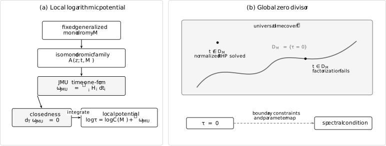
At fixed generalized monodromy $\mathcal M$, the JMU form is closed in the time directions and $\log\tau$ is its local scalar potential. The global zero divisor of $\tau$ records failure of the normalized inverse Riemann–Hilbert problem; a physical spectral condition requires additional boundary and parameter constraints.

Four poles select the bare matrix accessory

Work directly with a normalized Lax family having poles $0,t,1,\infty$, in which only $t$ moves. If one instead applies a time-dependent Möbius transformation to another family, the induced gauge and coordinate normalization can add an explicit exponent-dependent exact term. For the normalized family, the pairwise form immediately gives

$$\omega_{\mathrm{JMU}} = \left[ \frac{\operatorname{tr}(A_tA_0)}t + \frac{\operatorname{tr}(A_tA_1)}{t-1} \right]\dd t = H_t\,\dd t.$$

Thus

$$\frac{\dd}{\dd t}\log\tau=H_t.$$

Recall the notation fixed on the preceding page. The variables $(q,p)$ are spectral Darboux coordinates, and $q$ is the moving apparent singularity of the scalar reduction—not the Heun accessory $q_{\mathrm H}$. The quantities $a_t^{\mathrm{reg}}$, $\ell_t$, and $h_t$ record the regular scalar coefficient, Liouville-gauge residue, and local exponent convention used in that reduction.

The dictionary from the preceding page now becomes

$$\begin{aligned} \frac{\dd}{\dd t}\log\tau &= H_t \\ &= K_t - \frac{q(q-1)p}{t(t-1)} - \frac{\theta_\infty q}{2t(t-1)} - f(t) \\ &= -c_t^{\mathrm{sc}} - a_t^{\mathrm{reg}} + \left( h_t+\frac12 \right)\ell_t. \end{aligned}$$

The first line is the JMU convention. The second compensates for the explicitly time-dependent Darboux chart. The third compensates for cyclic scalar reduction and the Liouville gauge. Any use of a Painlevé Hamiltonian or a Heun accessory in a tau formula must include the relevant correction rather than silently relabeling it as $H_t$. The function $f(t)$ is the freedom to add a time-only term to the moving-chart Hamiltonian: it changes the chosen primitive by $\int f(t)\,\dd t$, so it is a Hamiltonian convention, not the time-independent JMU normalization constant.

Painlevé sigma conventions usually modify $t(t-1)\partial_t\log\tau$ by an affine, exponent-dependent function. A sigma equation is therefore not a convention-free replacement for the JMU identity; the precise affine shift used in this book is fixed on the next page.

The irreducible rational checkpoint fixes derivatives, not a value

For the exact tuple on the preceding page at $t=2$,

$$\left. \frac{\dd}{\dd t}\log\tau \right|_{t=2} = H_t = -\frac{31}{3}.$$

The two traces are

$$\operatorname{tr}(A_tA_0)=\frac{11}{3}, \qquad \operatorname{tr}(A_tA_1)=-\frac{73}{6}.$$

Since a Hamiltonian has zero bracket with itself, total differentiation along its own flow leaves only the explicit $t$-derivative:

$$\begin{aligned} \left. \frac{\dd H_t}{\dd t} \right|_{t=2} &= - \frac{\operatorname{tr}(A_tA_0)}{t^2} - \frac{\operatorname{tr}(A_tA_1)}{(t-1)^2} \\ &= \frac{45}{4}. \end{aligned}$$

Therefore $(\log\tau)''(2)=45/4$. Neither derivative determines $\tau(2)$: that value still depends on the multiplicative constant and on integration from a normalized base point.

Commuting residues give an exact tau benchmark

Suppose all residues commute. The Schlesinger commutators vanish, so the $A_i$ are constant while the poles move. On any patch with fixed logarithm branches,

$$\tau = C \prod_{i<j} (a_i-a_j)^{ \operatorname{tr}(A_iA_j) }.$$

Indeed, its logarithmic differential is the pairwise JMU form. For the four-pole normalization this reduces, up to a $t$-independent factor, to

$$\tau(t) = C\, t^{\operatorname{tr}(A_0A_t)} (t-1)^{\operatorname{tr}(A_tA_1)}.$$

Differentiating gives

$$\frac{\dd}{\dd t}\log\tau = \frac{\operatorname{tr}(A_tA_0)}t + \frac{\operatorname{tr}(A_tA_1)}{t-1}.$$

This benchmark is reducible and need not lie on the smooth generic character surface. Its purpose is narrower: it checks the factor of $1/2$, the ordering signs, the logarithm branches, and the normalization independence of the JMU differential.

The triangular benchmark is noncommuting but still integrable

The exactly solvable upper-triangular trajectory on the Schlesinger page has

$$h_0=\frac17, \qquad h_t=\frac16, \qquad h_1=\frac15.$$

Its commutators are nonzero, but $\operatorname{tr}(A_iA_j)=2h_ih_j$ remains constant because the strictly upper-triangular parts do not contribute to the trace. Hence

$$H_t = \frac{1}{21t} + \frac{1}{15(t-1)}, \qquad \tau(t) = C\, t^{1/21}(t-1)^{1/15}.$$

A positive circuit around $0$ or $1$ multiplies this representative by $\exp(2\pi\ii/21)$ or $\exp(2\pi\ii/15)$. These are branch multipliers, not zeros. The points $0$ and $1$ are collision boundaries of time space, not interior points of the Malgrange divisor.

Tau zeros form the Malgrange divisor

Let $\mathcal T$ be the collision-free time space and $\widetilde{\mathcal T}$ its universal cover. Fix generalized monodromy data $\mathcal M$ for which the normalized inverse Riemann–Hilbert problem is solvable at one base time. On the nonresonant semisimple locus declared above, the normalized problem reconstructs the rational connection in the chosen trivial-bundle chart away from an analytic divisor $\mathcal D_{\mathcal M}$.

The local exponential formula for tau cannot vanish on its regular patch. Zeros appear only after continuation toward a locus where that Riemann–Hilbert chart fails and $\omega_{\mathrm{JMU}}$ develops a logarithmic pole.

The Malgrange–Miwa continuation theorem extends the local tau function holomorphically to $\widetilde{\mathcal T}$. With the natural multiplicities, its zero divisor is exactly the inverse-problem failure divisor:

$$\mathcal D_{\mathcal M} = \operatorname{div}_0 \tau(\,\cdot\,;\mathcal M).$$

At such a point, the prescribed generalized monodromy data have not ceased to exist. Rather, the normalized Birkhoff–Riemann–Hilbert factorization fails, equivalently the associated holomorphic bundle is nontrivial in the declared trivial-bundle model. The Schlesinger residues therefore continue meromorphically and may leave the residue chart through a pole.

In one time, suppose $t_*$ is a zero of order $k$:

$$\tau(t) = (t-t_*)^k g(t), \qquad g(t_*)\ne0.$$

Then

$$H_t = \frac{\dd}{\dd t}\log\tau = \frac{k}{t-t_*} + \frac{g'(t)}{g(t)}.$$

Thus the logarithmic derivative has a simple pole with positive integer residue $k$. In several times, the corresponding statement is local and normal to a smooth component of the divisor.

Time normalization and monodromy normalization are different problems

The original JMU equation fixes time derivatives at one monodromy point:

$$\dd_{\mathcal T}\log\tau = \omega_{\mathrm{JMU}}.$$

If $\tau_1$ and $\tau_2$ obey this equation on the same connected isomonodromic leaf, then

$$\frac{\tau_1}{\tau_2}=C(\mathcal M).$$

This is the familiar multiplicative ambiguity. It becomes a genuine connection-constant problem when asymptotics at different critical points, different sectors, or different monodromy data are compared.

Simply allowing monodromy differentials in the uncorrected JMU expression does not generally produce a closed form on the full time–monodromy space. Malgrange- and Bertola-type constructions add a normalization-dependent monodromy one-form. Once a closed representative $\widehat\omega$ has been chosen,

$$\dd\log\widehat\tau=\widehat\omega$$

also controls relative normalization as $\mathcal M$ varies. This extended object should not be substituted into the original JMU formula without stating the added one-form and its gauge convention.

On the non-simply connected time space, the periods of $\omega_{\mathrm{JMU}}$ can produce multiplicative continuation factors. It is therefore safest to regard tau locally as a function and globally as a section of a line bundle, or to work on $\widetilde{\mathcal T}$ with a fixed marking and base normalization. Concretely, local representatives on overlapping charts obey

$$\tau_V=g_{VU}\tau_U, \qquad g_{VU}\ne0, \qquad \dd_{\mathcal T}\log g_{VU}=0.$$

This last equation applies when both representatives use the same JMU time form. If a change of trivialization also changes the representative form, the consistent transformation law is

$$\omega_V = \omega_U+\dd_{\mathcal T}\log g_{VU}.$$

Numerical values depend on the trivialization, while multiplication by the nowhere-zero transition factor leaves the common zero divisor unchanged.

JMU tau, Fredholm representations, and spectral determinants

Three uses of “determinant” must be separated:

Construction	What must be proved	Meaning of a zero
JMU or extended isomonodromic tau function	Its logarithmic differential is the declared JMU or extended form	Malgrange/Riemann–Hilbert obstruction
Fredholm determinant representation of tau	An operator identity identifies the determinant with tau up to an explicit nonzero factor	The same isomonodromic obstruction in that representation
Spectral determinant of an original scalar operator	Boundary data, analytic domain, regularization, and normalization define the spectrum	Eigenvalue, resonance, or another declared spectral condition

Some isomonodromic tau functions do admit Fredholm determinant representations. That is a theorem about a particular Riemann–Hilbert operator, not the definition of the JMU tau function. It does not make the Fredholm determinant the spectral determinant of the scalar equation from which a Lax pair may have been derived.

Likewise, a condition $\tau=0$ becomes a quantization or quasinormal-mode condition only after the physical boundary conditions have been translated into monodromy constraints and the spectral parameter has been embedded in the time/monodromy data. The inverse-monodromy and numerical pages later in this chapter perform those extra steps.

The next page makes the first bridge explicit for the four-pole Painlevé VI Lax system. Its scalar reduction still has the moving apparent pole $q$; a Heun equation appears only on a specified specialization, and the Heun accessory is related to $\partial_t\log\tau$ only after the scalar-reduction and gauge corrections above are applied.

Common pitfalls

Using the moving-chart Hamiltonian as the JMU derivative. In this chapter’s convention, $\partial_t\log\tau=H_t$. The generator $K_t$ contains explicit coordinate-drift terms and possibly $f(t)$.

Calling the multiplicative constant irrelevant. It is irrelevant for one time derivative, but essential for connection formulae and comparisons between different asymptotic regimes.

Reading a tau zero as loss of monodromy data. The monodromy point is fixed. What fails is the normalized inverse problem in the selected bundle chart.

Extending in monodromy directions without a correction. JMU closedness is a time-direction statement. A full-space extension needs an additional monodromy one-form and a declared normalization.

Equating every tau function with a spectral determinant. Boundary conditions and a parameter dictionary are indispensable. Without them, the two zero sets solve different problems.

Exercises

1. Recover one Fuchsian Hamiltonian

Use the local recursion at $a_i$ to prove $\operatorname{tr}(\Theta_i g_{i,1})=H_i$ and evaluate the corresponding JMU residue.

Solution

The constant term of the local differential equation is

$$B_i = G_i \left( g_{i,1}+[g_{i,1},\Theta_i] \right) G_i^{-1}.$$

Multiplication by $A_i=G_i\Theta_iG_i^{-1}$ and trace cyclicity give

$$\operatorname{tr}(A_iB_i) = \operatorname{tr}(\Theta_i g_{i,1}),$$

because $\operatorname{tr}(\Theta_i[g_{i,1},\Theta_i])=0$. The left side is

$$\operatorname{tr}(A_iB_i) = \sum_{j\ne i} \frac{\operatorname{tr}(A_iA_j)} {a_i-a_j} =H_i.$$

Finally,

$$\dd_{\mathcal T}\Theta_i(z) = -\frac{\Theta_i\,\dd a_i}{z-a_i},$$

so the outer minus sign in the JMU definition yields $H_i\,\dd a_i$.

2. Pass from residues to the pairwise form

Show directly that

$$\sum_iH_i\,\dd a_i = \sum_{i<j} \operatorname{tr}(A_iA_j) \, \dd\log(a_i-a_j).$$

Solution

For a fixed pair $i<j$,

$$\dd\log(a_i-a_j) = \frac{\dd a_i-\dd a_j}{a_i-a_j}.$$

Its contribution to the coefficient of $\dd a_i$ is $\operatorname{tr}(A_iA_j)/(a_i-a_j)$. If $j<i$, the two sign changes in the denominator and differential give the same expression. Summing over all partners of $i$ produces $H_i$.

3. Integrate a commuting Schlesinger family

Assume $[A_i,A_j]=0$ for every pair. Derive the product formula for tau and explain where branch choices enter.

Solution

Every Schlesinger right-hand side vanishes, so all residues are constant. Integrating the pairwise form gives

$$\log\tau = \log C + \sum_{i<j} \operatorname{tr}(A_iA_j) \log(a_i-a_j).$$

Exponentiation yields

$$\tau = C \prod_{i<j} (a_i-a_j)^{ \operatorname{tr}(A_iA_j) }.$$

Each power uses the chosen logarithm on a simply connected patch. Continuation around a collision can multiply tau by a nonzero constant.

4. Audit the exact four-pole slope

For the irreducible tuple at $t=2$, use

$$\operatorname{tr}(A_tA_0)=\frac{11}{3}, \qquad \operatorname{tr}(A_tA_1)=-\frac{73}{6}$$

to compute $(\log\tau)'$ and $(\log\tau)''$.

Solution

At $t=2$,

$$(\log\tau)' = \frac{11/3}{2} + \frac{-73/6}{1} = -\frac{31}{3}.$$

Because $\{H_t,H_t\}=0$,

$$\begin{aligned} (\log\tau)'' &= \frac{\dd H_t}{\dd t} \\ &= - \frac{11/3}{2^2} - \frac{-73/6}{1^2} = \frac{45}{4}. \end{aligned}$$

No value of $\tau(2)$ follows without fixing its multiplicative normalization.

5. Track an elementary change of tau representative

On a simply connected collision-free patch, define

$$\widetilde\tau(t) = \mathrm e^{\gamma t} t^\alpha (t-1)^\beta \tau(t).$$

Compute its logarithmic derivative and its continuation multipliers around $0$ and $1$. Does this factor change the interior zero divisor?

Solution

Direct differentiation gives

$$\frac{\dd}{\dd t}\log\widetilde\tau = H_t + \gamma + \frac{\alpha}{t} + \frac{\beta}{t-1}.$$

A positive circuit around $0$ multiplies the chosen representative by $\exp(2\pi\ii\alpha)$, while a positive circuit around $1$ multiplies it by $\exp(2\pi\ii\beta)$. The exponential factor is single-valued. All three elementary factors are nonzero at interior points of the collision-free patch, so they do not change the interior zero divisor. They do change the logarithmic differential, however, and therefore are not the time-independent JMU ambiguity unless $\gamma=\alpha=\beta=0$.

6. Read the multiplicity of a tau zero

Let $\tau(t)=(t-t_*)^kg(t)$ with $g(t_*)\ne0$. Show that the residue of $H_t=(\log\tau)'$ at $t_*$ is $k$.

Solution

Direct differentiation gives

$$H_t = \frac{k}{t-t_*} + \frac{g'(t)}{g(t)}.$$

The second term is holomorphic at $t_*$, so the pole is simple and its residue is the zero multiplicity $k$.

7. Test a proposed spectral interpretation

A calculation finds $\tau(t_*)=0$ and immediately calls $t_*$ an eigenvalue. List the missing statements needed to justify that conclusion.

Solution

One must specify:

1. the scalar operator and its analytic domain;
2. the boundary or outgoing conditions defining its spectrum;
3. the map from the spectral parameter to isomonodromic times and monodromy data;
4. the monodromy constraints equivalent to those boundary conditions;
5. a proof that the relevant boundary function is tau, or tau times an explicit factor that is nonzero on the domain of interest.

Without these steps, $\tau(t_*)=0$ states only that the normalized inverse Riemann–Hilbert problem lies on its Malgrange divisor.

8. Solve the scalar-accessory dictionary

Solve the four-pole dictionary for $c_t^{\mathrm{sc}}$. Why does the result not yet give the standard Heun accessory $q_{\mathrm H}$?

Solution

$$c_t^{\mathrm{sc}} = - \frac{\dd}{\dd t}\log\tau - a_t^{\mathrm{reg}} + \left( h_t+\frac12 \right)\ell_t.$$

This is the accessory residue of the scalar normal form obtained from the declared cyclic vector and Liouville gauge. Generically that scalar equation still contains the moving apparent pole at $z=q$. The standard Heun equation has only four regular singular points, and its accessory $q_{\mathrm H}$ is obtained only after a specified specialization or removal of the apparent pole together with a parameter and gauge dictionary. That bridge is constructed on the next page.

References

• M. Jimbo, T. Miwa, and K. Ueno, “Monodromy Preserving Deformation of Linear Ordinary Differential Equations with Rational Coefficients. I. General Theory and τ-Function”, Physica D 2 (1981), 306–352. Equation (5.1) gives the general JMU form; Example 5.1 gives the Fuchsian specialization.
• T. Miwa, “Painlevé Property of Monodromy Preserving Deformation Equations and the Analyticity of τ Functions”, Publications of the Research Institute for Mathematical Sciences 17 (1981), 703–721. Analyticity of tau and meromorphic continuation of the deformation variables.
• B. Malgrange, “Déformations isomonodromiques des singularités régulières”, Recherche Coopérative sur Programme 31 (1983), 1–26. The inverse-problem and bundle-theoretic origin of the divisor.
• J. Palmer, “Zeros of the Jimbo, Miwa, Ueno Tau Function”, Journal of Mathematical Physics 40 (1999), 6638–6681. Zeros of tau and failure of the Birkhoff–Riemann–Hilbert problem for irregular systems.
• P. Gavrylenko and O. Lisovyy, “Fredholm Determinant and Nekrasov Sum Representations of Isomonodromic Tau Functions”, Communications in Mathematical Physics 363 (2018), 1–58. Fredholm representations for generic Fuchsian $\operatorname{GL}(N,\mathbb C)$ systems, illustrating that a determinant formula is an additional representation theorem rather than the JMU definition.
• M. Bertola, “The Dependence on the Monodromy Data of the Isomonodromic Tau Function”, Communications in Mathematical Physics 294 (2010), 539–579, together with the correction. Malgrange differentials and monodromy-direction extensions.
• A. R. Its, O. Lisovyy, and A. Prokhorov, “Monodromy Dependence and Connection Formulae for Isomonodromic Tau Functions”, Duke Mathematical Journal 167 (2018), 1347–1432. Closed extensions, normalization constants, and the four-point Fuchsian case.