WKB Differentials and Homology

The square root $P_0=\sqrt{R_0}$ becomes the tautological one-form $\lambda_0$ on the normalized spectral cover. The same geometric upgrade applies coefficient by coefficient to the formal WKB phase. What remains is to declare where those one-forms are singular and which one-dimensional chains they may be integrated over.

That declaration matters. A closed cycle, an open path between turning points, and a path ending at a pole belong to different homological problems. A genus-zero cover can still carry a nonzero period after its poles are removed, and a point that is harmless for $\lambda_0$ can become a pole of the first quantum correction.

Page question

Which punctured and relative homology groups carry the classical and formal WKB actions, and how do sheet choice, orientation, and intersection number control their signs?

Status ledger

Statement	Status
$P_{\mathrm{even}}\,\dd z$ is a formal one-form	Exact formal identity with the half-density and Schwarzian conventions of Pages 1–2
Its coefficients are meromorphic upstairs	Coefficientwise statement on the normalized leading cover
Absolute and relative cycle groups	Topological after the punctures and allowed endpoints are declared
Classical actions and closed periods	Ordinary convergent integrals when paths avoid poles
Endpoint subtraction and all-orders periods	Deferred to Page 5
Borel sums, Stokes jumps, and exact quantization	Deferred to Chapter 9

The branch difference is a formal one-form

Keep the even-$\hbar$ setting of Page 2,

$$\hbar^2\psi'' = R(z,\hbar)\psi, \qquad R(z,\hbar) = R_0(z)+\hbar^2R_2(z)+\cdots.$$

For the two formal Riccati branches $P^{(\pm)}$, define

$$P_{\mathrm{even}} = \frac{P^{(+)}-P^{(-)}}2.$$

The formal WKB phase differential is

$$\begin{aligned} \Omega(\hbar) &:= P_{\mathrm{even}}(z,\hbar)\,\dd z \\ &= \sum_{k\geq0} \hbar^{2k}\lambda_{2k}, \qquad \lambda_{2k}:=p_{2k}(z)\,\dd z. \end{aligned}$$

Its leading coefficient is the form constructed on Page 3:

$$\lambda_0 = y\,\dd z, \qquad y^2=R_0(z).$$

In the traditional unscaled logarithmic-derivative convention,

$$S_{\mathrm{odd}}^{\mathrm{trad}}\,\dd z = \hbar^{-1}\Omega(\hbar).$$

This translation prevents a frequent one-power-of-$\hbar$ error when period formulas are compared across sources.

Under an $\hbar$-independent coordinate change $z=z(w)$, the inverse-half-density transformation and its Schwarzian correction give

$$\widetilde P_{\mathrm{even}}(w,\hbar)\,\dd w = P_{\mathrm{even}}(z,\hbar)\,\dd z.$$

Because the coordinate change does not mix powers of $\hbar$, every $\lambda_{2k}$ is a meromorphic one-form on the fixed leading cover $\widehat\Sigma$. The deck involution acts by

$$\tau^*\lambda_{2k} = -\lambda_{2k}.$$

If odd powers occur in $R$, the branch difference is still the intrinsic object, but its expansion need not contain even powers only. The notation $\lambda_{2k}$ on this page therefore always presumes the stated $\hbar$-parity hypothesis.

Every finite WKB order has its own punctures

There is no useful homology group until the removed divisor has been specified. At a truncation through $\hbar^{2N}$, set

$$D_N := \bigcup_{k=0}^{N} \operatorname{Pole}(\lambda_{2k}), \qquad X_N := \widehat\Sigma\setminus D_N.$$

The coefficients $\lambda_0,\ldots,\lambda_{2N}$ are holomorphic on $X_N$, so their integrals around closed contours depend only on homology classes in $X_N$. For meromorphic data on a compact cover, $D_N$ is finite. If all coefficient divisors lie in one fixed finite set, that larger set may be removed once and for all; this is an additional hypothesis, not automatic notation.

The classical punctures are

$$D_0 = \operatorname{Pole}(\lambda_0).$$

By Page 3, these lie above poles of the quadratic differential $\phi_0=R_0\,\dd z^2$ of order at least $2$. A simple zero of $\phi_0$ lifts to a zero of $\lambda_0$, and a simple pole of $\phi_0$ lifts to a regular nonzero point. Neither must be removed for a classical integral.

Higher WKB coefficients behave differently. For an $\hbar$-independent potential near a generic simple turning point, write

$$z-z_t=\xi^2.$$

The local estimate proved on Page 2 gives, for $k\geq1$,

$$\lambda_{2k} \sim C_{2k}\, \xi^{-(6k-2)}\,\dd\xi, \qquad C_{2k}\neq0.$$

Thus $\lambda_2$ already has a fourth-order pole upstairs. The turning point is a legitimate endpoint for the classical action but a puncture for the unregularized $\hbar^2$ coefficient. Page 5 will explain how regularization compares the resulting coefficientwise integrals.

Closed periods see the anti-invariant lattice

For a closed cycle

$$\gamma\in H_1(X_N,\mathbb Z),$$

define the coefficient period

$$\Pi_{\gamma,2k} := \oint_\gamma\lambda_{2k}, \qquad 0\leq k\leq N.$$

A holomorphic one-form on a Riemann surface is closed, so this pairing does not change under a deformation of $\gamma$ inside $X_N$. A deformation that crosses a removed pole is not an allowed homotopy in $X_N$. If $\ell_p$ is a small positively oriented loop around a pole $p$,

$$\oint_{\ell_p}\lambda_{2k} = 2\pi\ii\operatorname{Res}_p\lambda_{2k}.$$

Residues are therefore part of the period ledger, even when the compactified curve has no handles.

Anti-invariance gives

$$\Pi_{\tau_*\gamma,2k} = -\Pi_{\gamma,2k}.$$

Every invariant cycle has zero WKB period. A natural integral charge lattice at order $N$ is consequently

$$\Gamma_N^- := \ker\!\left( 1+\tau_*: H_1(X_N,\mathbb Z) \longrightarrow H_1(X_N,\mathbb Z) \right).$$

For the classical differential we abbreviate

$$\Gamma_{\mathrm{cl}} := H_1(X_0,\mathbb Z)^-.$$

An integral factor of two

Some exact-WKB sources quotient cycles by symmetric classes instead of taking the negative eigensublattice. Over $\mathbb Q$, the anti-invariant projection is

$$\gamma^-_{\mathbb Q} = \frac{\gamma-\tau_*\gamma}{2}.$$

Over $\mathbb Z$, division by $2$ may leave the lattice. The integral class $\gamma-\tau_*\gamma$ has twice the period of $\gamma$, and an already anti-invariant class maps to twice itself. State the lattice convention before importing a period formula.

Relative classes remember endpoints

Let $M\subset X_0$ be a finite set of allowed endpoints. An oriented open path $\beta$ from $p$ to $q$ defines

$$[\beta] \in H_1(X_0,M;\mathbb Z), \qquad \partial[\beta] = [q]-[p].$$

If $X_0$ is connected and $M$ is nonempty, the relevant part of the long exact sequence is

$$0 \longrightarrow H_1(X_0;\mathbb Z) \longrightarrow H_1(X_0,M;\mathbb Z) \xrightarrow{\ \partial\ } \widetilde H_0(M;\mathbb Z) \longrightarrow 0.$$

Consequently, two relative classes with the same ordered endpoints differ by a unique absolute homology class. For an endpoint set where $\lambda_0$ is regular, define

$$\mathcal A_\beta^{(0)} := \int_\beta\lambda_0.$$

If $\beta'=\beta+\gamma$, then

$$\mathcal A_{\beta'}^{(0)} = \mathcal A_\beta^{(0)} + \Pi_{\gamma,0}.$$

An open action is therefore an affine quantity over the lattice of closed periods. Changing the path used to normalize a WKB exponential multiplies its leading factor by

$$\exp\!\left( \pm\frac{\Pi_{\gamma,0}}{\hbar} \right).$$

Lifted turning points are valid members of $M$ for $\lambda_0$ because the classical form is finite there. A lift of a simple-pole branch point is also classically regular, although its exact-WKB local model is special. By contrast, an endpoint in $D_0$ is not made integrable merely by calling the chain relative. A cutoff, a local coordinate, and an endpoint subtraction are then required.

For readers comparing exact-WKB conventions, a common notation is

$$\begin{aligned} \widehat P_0 &= \pi^{-1}\{\text{zeros of }\phi_0\}, \\ \widehat P_\infty &= \pi^{-1}\{\text{poles of }\phi_0\}, \\ \widehat P &= \widehat P_0\cup\widehat P_\infty. \end{aligned}$$

Iwaki–Nakanishi use $H_1(\widehat\Sigma\setminus\widehat P)$ for cycles and $H_1(\widehat\Sigma\setminus\widehat P_0,\widehat P_\infty)$ for paths. Those groups are adapted to formal Voros symbols and their singular endpoints. They should not be silently identified with the smaller classical pair just defined.

A lifted branch arc closes with a factor of two

Let $a$ and $b$ be ramification points fixed by $\tau$, and let $\beta:a\to b$ be a lift of an oriented base arc on one sheet. Give $\tau_*\beta$ the induced orientation from $a$ to $b$ on the other sheet. Their boundaries agree, so

$$\delta_\beta := \beta-\tau_*\beta$$

is closed. It is anti-invariant:

$$\tau_*\delta_\beta = -\delta_\beta.$$

Let $\lambda$ be an anti-invariant one-form whose integral along $\beta$ converges at both endpoints. Then

$$\begin{aligned} \oint_{\delta_\beta}\lambda &= \int_\beta\lambda - \int_{\tau_*\beta}\lambda \\ &= 2\int_\beta\lambda. \end{aligned}$$

This is the source of the ubiquitous factor of two between a one-way turning-point action and the cycle surrounding the corresponding cut. It is not a mysterious normalization constant.

In particular, the identity is an ordinary convergent integral for $\lambda_0$ at simple turning points. At generic simple turning points, $\lambda_{2k}$ has a pole for $k\geq1$, so $\beta$ is not a chain in $X_N$ and neither raw integral above exists. Page 5 introduces compatible endpoint subtractions; only after that regularization may the same factor-of-two ledger be applied coefficient by coefficient.

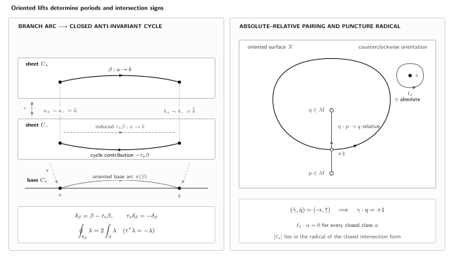
The homological ledger. A displayed cut is bookkeeping on the base; the closed cycle upstairs is $\delta_\beta=\beta-\tau_*\beta$. In the relative panel, ordered tangents at the marked crossing give intersection number $+1$, while the small puncture loop lies in the radical of the closed intersection form.

The construction assumes that both endpoints are fixed by the deck involution, as they are over odd-order branch values. An even-order zero has two distinct lifts. A path ending there must name the chosen preimage, and $\beta-\tau_*\beta$ need not close without additional connecting data.

The complete elementary sign ledger is

$$\begin{aligned} \Pi_{-\gamma,2k} &= -\Pi_{\gamma,2k}, \\ \Pi_{\tau_*\gamma,2k} &= -\Pi_{\gamma,2k}, \\ \Pi_{-\tau_*\gamma,2k} &= \Pi_{\gamma,2k}. \end{aligned}$$

Reversing the orientation and changing sheets are two separate sign operations; doing both leaves a WKB period unchanged.

Intersection numbers fix the orientation ledger

Put two oriented curves in transverse position. A crossing contributes $+1$ when the ordered tangent vectors of the first and second curves agree with the complex orientation of $\widehat\Sigma$, and $-1$ otherwise. The resulting intersection number is skew:

$$\gamma\mathbin{\cdot}\delta = -\delta\mathbin{\cdot}\gamma.$$

For a compact genus-$g$ surface, a symplectic basis obeys

$$\begin{aligned} A_i\mathbin{\cdot}B_j &= \delta_{ij}, \\ A_i\mathbin{\cdot}A_j &= B_i\mathbin{\cdot}B_j = 0. \end{aligned}$$

There is no preferred object called “the $A$-period” before a basis is chosen. A matrix in $\operatorname{Sp}(2g,\mathbb Z)$ transforms the cycle column and its period column by the same integral linear rule.

Punctures change this familiar picture. If a connected genus-$g$ surface has $n>0$ punctures, then

$$\operatorname{rank}H_1 = 2g+n-1.$$

Small positive loops $\ell_1,\ldots,\ell_n$ around the punctures obey

$$\ell_1+\cdots+\ell_n=0.$$

Their $n-1$ independent classes have zero intersection with every closed class. They span the radical of the full punctured-surface intersection form. A symplectic basis describes the handle sector, or the quotient by this radical, but not the entire punctured lattice.

Absolute cycles and open paths also pair. If $M$ is the endpoint set, one convenient version is

$$H_1(X_0\setminus M;\mathbb Z) \times H_1(X_0,M;\mathbb Z) \longrightarrow \mathbb Z.$$

It counts transverse interior crossings while cycles avoid the relative endpoints. Puncturing those endpoints on the cycle side does not alter classical periods: a small loop around a point where $\lambda_0$ is holomorphic has zero integral. There is no equally automatic canonical relative–relative intersection pairing; endpoint conventions would have to be added.

Airy and Weber separate open and puncture actions

For Airy,

$$R_0(z)=z, \qquad z=\xi^2, \qquad \lambda_0=2\xi^2\,\dd\xi.$$

The compact cover is a sphere and $\lambda_0$ has one pole, at $\xi=\infty$. Removing it leaves a plane, so

$$\Gamma_{\mathrm{cl}}=0.$$

There is no nonzero closed classical period. There is nevertheless a finite relative action from the turning point to a regular point:

$$\int_0^z\lambda_0 = \frac23z^{3/2}$$

on a chosen sheet. It changes sign on the other sheet. Extending that path to infinity diverges.

For Weber, take

$$R_0(z)=z^2-a^2, \qquad a>0.$$

Let $\beta$ run from $-a$ to $a$ on the sheet

$$y=+\ii\sqrt{a^2-z^2}.$$

Then

$$\mathcal A_\beta^{(0)} = \ii \int_{-a}^{a} \sqrt{a^2-z^2}\,\dd z = \frac{\ii\pi a^2}{2},$$

and

$$\Pi_{\delta_\beta,0} = \ii\pi a^2.$$

The compact Weber cover also has genus $0$, so this cycle is null homologous on the compact sphere. But $\lambda_0$ has poles at the two points $\infty_\pm$. Hence

$$H_1\!\left( \widehat\Sigma\setminus\{\infty_+,\infty_-\}, \mathbb Z \right) \cong \mathbb Z,$$

and the cut cycle separates the two punctures. On the sheet with $y\sim z$, put $w=1/z$. The local expansion is

$$\lambda_0 = \left( -w^{-3} + \frac{a^2}{2}w^{-1} + O(w) \right) \dd w.$$

A positive small loop has period $\ii\pi a^2$, matching the cut-cycle period with a compatible orientation. Genus zero does not mean period zero once the differential is meromorphic.

In a real allowed region, the book convention $R_0=V-E$ gives

$$\lambda_0 = +\ii\sqrt{E-V(z)}\,\dd z$$

on the chosen sheet. Thus, for the cycle through real turning points $z_-<z_+$,

$$J_{\mathrm{cl}} := -\ii\Pi_{\delta_\beta,0} = 2 \int_{z_-}^{z_+} \sqrt{E-V(z)}\,\dd z$$

is the usual positive full-orbit mechanical action. The imaginary WKB period is a consequence of the $V-E$ convention, not a sign error.

The generic Mathieu curve will add a genuine genus-one pair with $A\mathbin{\cdot}B=1$ on Page 7. It therefore separates handle periods from the residue direction seen in Weber.

Gauss–Manin transport moves the cycle with the curve

Let the energy vary away from the discriminant and from pole collisions. The groups

$$H_1(X_{0,E},\mathbb Z)$$

form a local system over that regular parameter domain. A symbol $\gamma(E)$ in a period formula denotes a Gauss–Manin-flat class. It does not mean that a contour drawn in one affine $z$-plane is held rigid while its branch points move through it.

For

$$y^2=V(z)-E$$

and a flat closed class,

$$\begin{aligned} \frac{\dd}{\dd E} \Pi_{\gamma,0}(E) &= \frac{\dd}{\dd E} \oint_{\gamma(E)}y\,\dd z \\ &= -\frac12 \oint_{\gamma(E)} \frac{\dd z}{y}. \end{aligned}$$

For an open action between finite simple turning points, the same formula holds locally: the moving-endpoint terms vanish because $y=0$ at both endpoints, and $\dd z/y$ is integrable there. It fails without modification at a singular endpoint or across the discriminant. This derivative identity is the bridge to the Picard–Fuchs method on Page 6.

In the Weber family $a^2=E$,

$$\Pi_{\delta,0}(E) = \ii\pi E, \qquad \frac{\dd\Pi_{\delta,0}}{\dd E} = \ii\pi.$$

The right side of the derivative formula gives the same value because

$$\oint_\delta\frac{\dd z}{y} = -2\pi\ii$$

with the orientation used above.

A vanishing cycle detects the discriminant

Near a nondegenerate collision, choose a local parameter $\mu$ so that

$$R_0(z;\mu) = c\left[ (z-z_c)^2-\mu \right] + \cdots, \qquad c\neq0.$$

The two branch points lie at $z_c\pm\sqrt\mu+\cdots$. Lift the short arc between them and close it by the deck transform. The resulting anti-invariant class $\delta(\mu)$ pinches at $\mu=0$ and is called a vanishing cycle. With the branch

$$\sqrt{R_0} = \ii\sqrt c\, \sqrt{\mu-(z-z_c)^2}$$

along the short segment,

$$\Pi_{\delta,0}(\mu) = \ii\pi\sqrt c\,\mu + O(\mu^{3/2}).$$

Thus its classical period vanishes linearly in the smoothing parameter. The topology and the period both signal the discriminant, but they do not select a Stokes direction.

If a positive parameter loop produces the positive Dehn twist about $\delta$, fix the Picard–Lefschetz sign by

$$T_\delta(\gamma) = \gamma - (\gamma\mathbin{\cdot}\delta)\delta.$$

The period vector undergoes the same integral shear. Reversing the parameter-loop convention reverses the twist. This is geometric monodromy of the family, not a Stokes automorphism of Borel sums.

Higher WKB coefficients become increasingly singular as the branch points merge. The fact that $\Pi_{\delta,0}\to0$ therefore does not justify termwise conclusions about a full formal or resummed period. A uniform local model is needed at the collision.

What topology does not yet supply

The constructions on this page determine:

• meromorphic coefficient one-forms on the leading cover;
• their finite-order puncture divisors;
• absolute, relative, and anti-invariant homology classes;
• intersection numbers and changes of basis;
• convergent classical actions and coefficientwise closed integrals;
• Gauss–Manin transport and geometric vanishing cycles.

They do not determine:

• a preferred cut system or a preferred $A$/$B$ basis;
• endpoint counterterms or logarithm branches at poles;
• a Stokes graph or a phase of $\hbar$;
• Borel summability, lateral sums, or Stokes automorphisms;
• boundary conditions or a quantization rule;
• a canonical analytic solution.

Page 5 fixes the all-orders and endpoint-regularization conventions. Page 6 turns parameter derivatives into differential equations for periods. Page 7 computes the Airy, Weber, and Mathieu models in detail. Chapter 9 begins only after these formal and topological ledgers are complete.

Reproducible action audit

The homology-action check verifies the Airy primitive, Weber open and closed actions, residues at both points over infinity, the Gauss–Manin derivative, and representative integral symplectic basis changes. Run

python3 public/code/advanced-ode/wkb-homology-action-check.py

The script checks algebraic and analytic identities. It does not pretend to prove a topological homology statement by symbolic calculation.

Common pitfalls

Drawing only on the base. A projected contour does not specify a WKB cycle. Record its lift, sheet changes, endpoints, and orientation.

Calling the branch cut a cycle. A cut is a drawing convention. The intrinsic closed class is assembled from oriented lifts on the normalized cover.

Using compact homology for a meromorphic form. Removing poles can create residue cycles and make the intersection form degenerate. The Weber period is the simplest counterexample.

Treating relative as synonymous with convergent. Relative homology records allowed boundaries. An integral ending at a pole still needs local subtraction data.

Calling the punctured pairing symplectic. Small puncture loops lie in its radical. Pass to the handle sector or the nondegenerate quotient before choosing a symplectic basis.

Freezing a drawn contour while parameters vary. Period differentiation transports a homology class by the Gauss–Manin connection. A fixed affine sketch can be crossed by moving branch points even when the transported class remains regular.

Exercises

1. Close a branch-point arc

Let $\beta$ join two ramification points fixed by $\tau$. Prove that

$$\delta_\beta = \beta-\tau_*\beta$$

is closed and anti-invariant. If $\lambda$ is anti-invariant and its integral along $\beta$ converges at both endpoints, compute the period of $\delta_\beta$ in terms of the one-way action.

Solution

Both paths have the same boundary,

$$\partial\beta = [b]-[a] = \partial(\tau_*\beta).$$

Therefore $\partial\delta_\beta=0$. Applying the involution gives

$$\tau_*\delta_\beta = \tau_*\beta-\beta = -\delta_\beta.$$

For an anti-invariant one-form $\lambda$,

$$\int_{\tau_*\beta}\lambda = \int_\beta\tau^*\lambda = -\int_\beta\lambda.$$

Hence

$$\oint_{\delta_\beta}\lambda = 2\int_\beta\lambda.$$

2. Recover the Weber period from a residue

For $y^2=z^2-a^2$, evaluate the open action from $-a$ to $a$ on the sheet $y=+\ii\sqrt{a^2-z^2}$. Then compute the residue of $\lambda_0=y\,\dd z$ at the point over infinity with $y\sim z$.

Solution

The area of a semicircle gives

$$\int_{-a}^{a} \sqrt{a^2-z^2}\,\dd z = \frac{\pi a^2}{2}.$$

Thus the open and doubled actions are

$$\mathcal A_\beta^{(0)} = \frac{\ii\pi a^2}{2}, \qquad \Pi_{\delta_\beta,0} = \ii\pi a^2.$$

With $w=1/z$ and $y\sim z$,

$$\begin{aligned} y &= w^{-1} - \frac{a^2}{2}w + O(w^3), \\ \dd z &= -w^{-2}\,\dd w. \end{aligned}$$

Therefore

$$\operatorname{Res}_{\infty_+}\lambda_0 = \frac{a^2}{2},$$

and a positive local loop has integral $2\pi\ii(a^2/2)=\ii\pi a^2$. The other point has the opposite residue.

3. Show that open paths form a torsor

Let $X$ be connected and let $p,q\in M\subset X$. Show that the set of relative classes with boundary $[q]-[p]$ is a torsor under $H_1(X;\mathbb Z)$.

Solution

In the exact sequence

$$0 \longrightarrow H_1(X) \longrightarrow H_1(X,M) \xrightarrow{\partial} \widetilde H_0(M) \longrightarrow 0,$$

the difference of two classes with the same boundary lies in $\ker\partial$, which is the image of $H_1(X)$. The first arrow is injective, so that absolute class is unique. Adding any absolute class preserves the boundary. The action is therefore free and transitive.

4. Find the puncture radical

Remove $n>0$ points from a compact connected genus-$g$ surface. Find the rank of its first homology and describe the radical of the intersection form.

Solution

A standard cell decomposition, or Euler characteristic, gives

$$\operatorname{rank}H_1 = 2g+n-1.$$

There are $2g$ handle generators and $n$ small puncture loops subject to the single relation

$$\ell_1+\cdots+\ell_n=0.$$

Every $\ell_j$ can be kept in a small disc disjoint from any chosen closed representative, so its intersection with every class is zero. The $n-1$ independent puncture loops span the radical. The remaining $2g$-dimensional quotient has the usual symplectic pairing.

5. Shear a symplectic basis

Suppose $A\mathbin{\cdot}B=1$. For $k\in\mathbb Z$, set

$$A'=A, \qquad B'=B+kA.$$

Verify that the pairing is preserved and determine the transformed periods.

Solution

Skew-symmetry gives $A\mathbin{\cdot}A=0$, so

$$A'\mathbin{\cdot}B' = A\mathbin{\cdot}(B+kA) = 1.$$

Linearity of integration gives

$$\Pi_{A',0} = \Pi_{A,0}, \qquad \Pi_{B',0} = \Pi_{B,0} + k\Pi_{A,0}.$$

The names of the periods change with the integral basis, while the period homomorphism itself does not.

6. Differentiate the Weber vanishing period

For

$$y^2=z^2-E,$$

use the cut-cycle orientation of the text to verify

$$\frac{\dd\Pi_{\delta,0}}{\dd E} = -\frac12 \oint_\delta\frac{\dd z}{y}.$$

What changes at $E=0$?

Solution

For $E>0$, the chosen period is

$$\Pi_{\delta,0} = \ii\pi E,$$

so its derivative is $\ii\pi$. On the upper lift of the cut, $y=+\ii\sqrt{E-z^2}$ and

$$\int_{-\sqrt E}^{\sqrt E} \frac{\dd z}{y} = -\ii\pi.$$

The deck-transformed lift contributes the opposite integral, and the minus sign in $\delta=\beta-\tau_*\beta$ doubles the result:

$$\oint_\delta\frac{\dd z}{y} = -2\pi\ii.$$

Multiplication by $-1/2$ gives $\ii\pi$. At $E=0$ the two branch points collide, the cycle pinches, and the smooth-fiber homology local system does not extend as an unchanged cycle lattice through that fiber. The finite limiting derivative does not remove this topological degeneration.

References

• T. Bridgeland and I. Smith, “Quadratic Differentials as Stability Conditions”, Publications Mathématiques de l’IHÉS 121 (2015), 155–278, §§2.3–2.4 and 3.2. Defines the spectral cover, anti-invariant hat homology, period map, residue directions, and intersection form.
• K. Iwaki and T. Nakanishi, “Exact WKB Analysis and Cluster Algebras”, Journal of Physics A: Mathematical and Theoretical 47 (2014), 474009, §§2.3–2.4, 3.1, and 6.4. Gives the cycle/path groups, intersection conventions, anti-invariant WKB form, and quotient convention used for Voros symbols.
• K. Iwaki, “Les Houches Lectures on Exact WKB Analysis and Painlevé Equations”, arXiv:2512.17599v2, May 2026, §§1.1.2 and 1.4. Develops the spectral curve, WKB periods, and the Weber absolute/relative examples in a modern convention.
• E. Delabaere, H. Dillinger, and F. Pham, “Résurgence de Voros et périodes des courbes hyperelliptiques”, Annales de l’Institut Fourier 43 (1993), 163–199. Foundational treatment of hyperelliptic periods and their exact-WKB role.
• A. Hatcher, Algebraic Topology, Cambridge University Press, 2002, §2.1 and §3.3. Provides the long exact sequence of a pair, intersection pairing, and duality used for absolute and relative classes.
• J. Carlson, S. Müller-Stach, and C. Peters, Period Mappings and Period Domains, second edition, Cambridge Studies in Advanced Mathematics 168, Cambridge University Press, 2017, Chapter 1, §1.1, equation (1.13). Fixes the Picard–Lefschetz sign convention used for the geometric monodromy statement.