Classical Blocks and Accessory Parameters at c → ∞

A classical conformal block is not obtained by setting a large number for the central charge in one ordinary block coefficient. One must scale the external and internal weights with the central charge, take the logarithm of the complete block, and only then extract the leading heavy term. The logarithm is essential: powers that diverge separately cancel into finite connected coefficients.

This page turns that prescription into a calculation. Starting from finite-level Virasoro Gram matrices, it derives the unit-leading classical block through level two, restores the channel power, and differentiates to obtain the four-pole oper accessory. An exact affine conversion then gives the standard Heun parameter. A rational example is checked a second way by integrating the oper around the fused pair and measuring its composite trace.

Regime lock

This page uses one heavy block branch as $b\to0$. There is no Fourier sum over shifted internal weights. The analytic $c_{\mathrm{Vir}}=1$ Fourier family on the previous page is a different construction with a different output.

What is established, and what remains local

Statement	Status
Finite-$b$ Virasoro Gram-matrix coefficients	Exact away from the relevant Kac divisors
Generic four-point semiclassical exponentiation	Proved as a sewing-series statement
The coefficientwise small-$t$ classical accessory germ	Locally convergent and locally unique under generic nondegeneracy assumptions
Heavy–light BPZ reduction to the oper	Exact at leading order once the derivative-compatible factorization exists
Continuation of one branch throughout the punctured $t$-plane	Not implied by the sewing-series theorem
A normalized Heun connection matrix from the accessory alone	Not supplied

The last two qualifications matter. Coefficientwise exponentiation does not make a chosen classical branch globally single-valued, and differentiating a pointwise asymptotic limit requires additional control.

Scale a block family before taking its logarithm

Put

$$h:=b^2, \qquad c_{\mathrm{Vir}} = \frac6h+13+6h.$$

For the four external labels and the internal $0t$ channel, choose the centered heavy lift

$$a_{\mathrm L,j} = \frac{\theta_j}{2b}, \qquad j\in \left\{ 0,t,1,\infty,0t \right\}.$$

Define the classical weights

$$\delta_j := \frac{1-\theta_j^2}{4}.$$

The corresponding finite-$b$ conformal weights are

$$\Delta_j = \frac{\delta_j}{h} +\frac12 +\frac h4.$$

Subleading $O(1)$ changes of the finite-$b$ lift do not alter the leading classical block, but they can alter the next semiclassical order. The same lift must therefore be used consistently when finite corrections or normalized probe solutions are later required.

Use the $0t$-channel normalization

$$\mathcal V_{0t}(t) = t^{ \Delta_{0t}-\Delta_0-\Delta_t } \widehat{\mathcal V}_{0t}(t),$$

with

$$\widehat{\mathcal V}_{0t}(t) = 1+\sum_{N\ge1}\mathcal V_N(h)t^N.$$

Fix a branch of $\Log t$, all five exponent lifts, and the OPE channel. The full and unit-leading classical blocks are

$$\begin{aligned} f_{0t}(t) &:= \lim_{h\to0} h\Log\mathcal V_{0t}(t), \\ \widehat f_{0t}(t) &:= \lim_{h\to0} h\Log\widehat{\mathcal V}_{0t}(t). \end{aligned}$$

For the formal sewing expansion, these limits are taken coefficient by coefficient after the logarithm is formed. Let

$$d:=\delta_{0t}, \qquad \kappa := d-\delta_0-\delta_t.$$

Then

$$f_{0t}(t) = \kappa\Log t +\widehat f_{0t}(t).$$

The distinction between these two normalizations is operational. The unit-leading block has an ordinary power-series germ; the full block has the logarithm whose derivative creates the singular part of the accessory.

Three limits that must not be conflated

1. The coefficientwise limit of $h\Log\widehat{\mathcal V}_{0t}$ defines a formal small-$t$ classical series.
2. Local convergence gives an analytic germ in a nonzero disk for generic data.
3. Analytic continuation of that germ along a path can meet singularities or branch points; varying the weights can additionally meet Kac divisors in parameter space.

Only the first operation is needed to derive the coefficients below. The second justifies evaluating the germ for sufficiently small $t$. The third requires a declared continuation path and cannot be inferred from the first two.

The logarithm isolates connected classical coefficients

Write

$$\Log\widehat{\mathcal V}_{0t}(t) = \sum_{N\ge1}\ell_N(h)t^N$$

and

$$\widehat f_{0t}(t) = \sum_{N\ge1}f_Nt^N.$$

The classical coefficients are

$$f_N = \lim_{h\to0}h\,\ell_N(h).$$

Differentiating $\widehat{\mathcal V}=\exp(\sum_{N\ge1}\ell_Nt^N)$ gives the exact finite-$b$ recursion

$$\ell_N = \mathcal V_N -\frac1N \sum_{k=1}^{N-1} k\,\ell_k\mathcal V_{N-k}.$$

The first three cases are

$$\begin{aligned} \ell_1 &= \mathcal V_1, \\ \ell_2 &= \mathcal V_2 -\frac12\mathcal V_1^2, \\ \ell_3 &= \mathcal V_3 -\mathcal V_1\mathcal V_2 +\frac13\mathcal V_1^3. \end{aligned}$$

Typically,

$$\mathcal V_N = O(h^{-N}),$$

whereas

$$\ell_N = O(h^{-1}).$$

The apparently stronger divergences cancel only in the connected combination. Numerically taking $h\to0$ in $\mathcal V_N$ first is therefore ill-conditioned and mathematically wrong. Form the logarithmic coefficient exactly—or with enough guard precision to resolve the cancellation—before multiplying by $h$.

A stable extraction test

At a sequence $h_j\to0$:

1. compute the finite-$b$ coefficients $\mathcal V_1,\ldots,\mathcal V_N$;
2. form $\ell_N$ by the recursion above;
3. inspect $h_j\ell_N(h_j)$;
4. repeat at increased arithmetic precision;
5. fit the residual to a regular expansion in $h_j$ only after the precision study is stable.

For the centered lift, the leading correction is usually regular in $h=b^2$. Near a singular Gram determinant, no such fit should be trusted without a separate limiting analysis.

Gram matrices make the first two levels explicit

Label the standard Virasoro descendant basis at level $N$ by partitions of $N$. The exact unit-leading coefficient has the form

$$\mathcal V_N = \boldsymbol\gamma_{\mathrm R}^{(N)\mathsf T} \left( G_\Delta^{(N)} \right)^{-1} \boldsymbol\gamma_{\mathrm L}^{(N)}.$$

Here $G_\Delta^{(N)}$ is the level-$N$ Gram matrix of the internal Verma module, while the two three-point vectors encode the external weights on the two pairs of pants. This formula is finite-$b$ representation theory; the classical limit enters only afterward.

Level one

At level one,

$$G_\Delta^{(1)} = 2\Delta,$$

and the two three-point matrix elements are

$$\begin{aligned} A_b &:= \Delta+\Delta_t-\Delta_0, \\ B_b &:= \Delta+\Delta_1-\Delta_\infty. \end{aligned}$$

Therefore

$$\mathcal V_1 = \frac{A_bB_b}{2\Delta}.$$

Introduce their classical numerators

$$\begin{aligned} A &:= d+\delta_t-\delta_0, \\ B &:= d+\delta_1-\delta_\infty. \end{aligned}$$

Since $\Delta=d/h+O(1)$,

$$f_1 = \lim_{h\to0}h\mathcal V_1 = \frac{AB}{2d}, \qquad d\neq0.$$

This is the first regular term in the unit-leading classical block, not the complete accessory. The channel pole $\kappa/t$ still has to be restored.

Level two

Use the ordered basis

$$\left( L_{-2}\lvert\Delta\rangle, L_{-1}^2\lvert\Delta\rangle \right).$$

The exact Gram matrix is

$$G_\Delta^{(2)} = \begin{pmatrix} 4\Delta+c_{\mathrm{Vir}}/2 & 6\Delta \\ 6\Delta & 4\Delta(2\Delta+1) \end{pmatrix}.$$

Define

$$\begin{aligned} P_b &:= \Delta+2\Delta_t-\Delta_0, & Q_b &:= \Delta+2\Delta_1-\Delta_\infty. \end{aligned}$$

The two descendant vectors are

$$\boldsymbol\gamma_{\mathrm L}^{(2)} = \begin{pmatrix} P_b \\ A_b(A_b+1) \end{pmatrix}, \qquad \boldsymbol\gamma_{\mathrm R}^{(2)} = \begin{pmatrix} Q_b \\ B_b(B_b+1) \end{pmatrix}.$$

Thus

$$\mathcal V_2 = \begin{pmatrix} Q_b & B_b(B_b+1) \end{pmatrix} \left( G_\Delta^{(2)} \right)^{-1} \begin{pmatrix} P_b \\ A_b(A_b+1) \end{pmatrix}.$$

Set

$$P := d+2\delta_t-\delta_0, \qquad Q := d+2\delta_1-\delta_\infty.$$

Expanding the exact inverse matrix and only then taking $h(\mathcal V_2-\mathcal V_1^2/2)$ gives

$$\begin{aligned} f_2 ={}& \frac{1}{ 16d^3(4d+3) } \left[ 16d^3PQ \right. \\ &\left. \quad -12d^2 \left( A^2Q+B^2P \right) \right. \\ &\left. \quad +2d(4d+3)AB(A+B) \right. \\ &\left. \quad +(5d-3)A^2B^2 \right]. \end{aligned}$$

The formula is generic at this level:

$$d\neq0, \qquad 4d+3\neq0.$$

In terms of the internal exponent, these excluded factors occur at

$$\theta_{0t}^2=1, \qquad \theta_{0t}^2=4.$$

They are singular loci of the generic inverse-Gram formula. A finite special block, logarithmic limit, or truncated module can still exist, but it must be constructed by assembling the appropriate expression before the limit rather than by substituting into the displayed rational formula.

Why the level-two formula is a useful audit

The leading $h^{-2}$ part of $\mathcal V_2$ equals $\mathcal V_1^2/2$. Its exact cancellation is the first nontrivial test of classical exponentiation. A code path that does not reproduce that cancellation is not computing the classical block.

Differentiation turns the block jet into an oper

At fixed external weights, fixed internal lift, and fixed analytic branch,

$$c_t^{\mathrm{op}} = \partial_t f_{0t}.$$

The small-$t$ jet is therefore

$$c_t^{\mathrm{op}} = \frac{\kappa}{t} +f_1 +2f_2t +O(t^2).$$

The four-pole normal-form equation is

$$\left[ \partial_z^2 +T_{\mathrm{op}}(z;t) \right]\psi(z) = 0,$$

where

$$\begin{aligned} T_{\mathrm{op}}(z;t) ={}& \frac{\delta_0}{z^2} + \frac{\delta_t}{(z-t)^2} + \frac{\delta_1}{(z-1)^2} \\ &+ \frac{\Lambda}{z(z-1)} + \frac{ t(t-1)c_t^{\mathrm{op}} }{ z(z-1)(z-t) }, \end{aligned}$$

and

$$\Lambda := \delta_\infty -\delta_0 -\delta_t -\delta_1.$$

If instead the equation is written in partial fractions,

$$\begin{aligned} T_{\mathrm{op}}(z;t) ={}& \frac{\delta_0}{z^2} + \frac{\delta_t}{(z-t)^2} + \frac{\delta_1}{(z-1)^2} \\ &+ \frac{c_0}{z} + \frac{c_t}{z-t} + \frac{c_1}{z-1}, \end{aligned}$$

the two constraints at infinity give

$$\begin{aligned} c_0 &= -\Lambda+(t-1)c_t, \\ c_1 &= \Lambda-tc_t. \end{aligned}$$

Thus one block derivative reconstructs all three finite residues.

The sewing annulus checks the channel pole

In the overlap region

$$|t|\ll|z|\ll1,$$

the pair of punctures must look like the selected intermediate primary. Using only the leading accessory term,

$$\begin{aligned} T_{\mathrm{op}}(z;t) &= \frac{ \delta_0+\delta_t+\kappa }{z^2} + O\left(\frac{t}{z^3}\right) + O\left(\frac1z\right) \\ &= \frac{d}{z^2} + O\left(\frac{t}{z^3}\right) + O\left(\frac1z\right). \end{aligned}$$

Dropping the OPE contribution $\kappa/t$ would leave the wrong fused double-pole coefficient. This check is independent of the level-one and level-two descendant calculation.

The internal channel fixes one composite conjugacy class

The scalar-oper powers associated with the fused channel are

$$\frac{1\pm\theta_{0t}}2.$$

For the natural determinant-one scalar lift,

$$\operatorname{tr}(M_0M_t) = -2\cos(\pi\theta_{0t}).$$

The trace is periodic under

$$\theta_{0t} \longmapsto \pm\theta_{0t}+2m, \qquad m\in\mathbb Z,$$

but the lifted block data are not. Apart from the sign pair, $d=(1-\theta_{0t}^2)/4$, the OPE power, and the accessory branch generally change. One must therefore fix an exponent lift before computing the classical block, rather than reduce $\theta_{0t}$ modulo the trace periodicity at the start.

Chapter 5 uses a traceless-system lift with

$$\operatorname{tr}(M_0M_t) = 2\cos(\pi\sigma_{0t}).$$

For the same ordered separating loop,

$$\sigma_{0t} \equiv 1\pm\theta_{0t} \pmod2.$$

The central sign is a scalar-versus-system lift, not a disagreement about projective monodromy.

The internal channel fixes only this conjugacy class and its lift. A complete point of the four-puncture character variety also contains a conjugate twist coordinate. Locally, a normalized generating function

$$W(\theta_{0t},t) = W_0(\theta_{0t}) +f_{0t}(\theta_{0t},t)$$

can satisfy

$$\partial_tW=c_t, \qquad \partial_{\theta_{0t}}W=\mu_{0t}.$$

The $t$-independent term $W_0$ does not change the oper accessory, but it does change the normalization of the twist $\mu_{0t}$. This is why one fixed internal weight is not the same thing as complete monodromy data.

The standard Heun parameter is affine, not the derivative

Use the standard general-Heun equation

$$\begin{aligned} y''(z) &+ \left( \frac{\gamma_{\mathrm H}}z + \frac{\delta_{\mathrm H}}{z-1} + \frac{\epsilon_{\mathrm H}}{z-t} \right)y'(z) \\ &+ \frac{ \alpha_{\mathrm H}\beta_{\mathrm H}z-q_{\mathrm H} }{ z(z-1)(z-t) }y(z) = 0. \end{aligned}$$

Choose the positive exponent representatives

$$\begin{aligned} \gamma_{\mathrm H} &= 1-\theta_0, & \delta_{\mathrm H} &= 1-\theta_1, & \epsilon_{\mathrm H} &= 1-\theta_t, \\ \alpha_{\mathrm H} &= 1-\frac{ \theta_0+\theta_1+\theta_t-\theta_\infty }{2}, \\ \beta_{\mathrm H} &= 1-\frac{ \theta_0+\theta_1+\theta_t+\theta_\infty }{2}. \end{aligned}$$

They obey the Fuchs relation

$$\gamma_{\mathrm H} +\delta_{\mathrm H} +\epsilon_{\mathrm H} = \alpha_{\mathrm H} +\beta_{\mathrm H} +1.$$

The local scalar gauge

$$\begin{aligned} y(z) ={}& z^{-\gamma_{\mathrm H}/2} (1-z)^{-\delta_{\mathrm H}/2} \\ &\times \left( 1-\frac zt \right)^{-\epsilon_{\mathrm H}/2} \psi(z) \end{aligned}$$

gives the exact affine conversion

$$\begin{aligned} q_{\mathrm H} ={}& \frac{\gamma_{\mathrm H}}2 \left( t\delta_{\mathrm H} +\epsilon_{\mathrm H} \right) +t\Lambda \\ &- t(t-1)c_t^{\mathrm{op}}. \end{aligned}$$

Substituting the accessory jet gives

$$q_{\mathrm H}(t) = q_0+q_1t+q_2t^2+O(t^3),$$

where

$$\begin{aligned} q_0 &= \frac{ \gamma_{\mathrm H}\epsilon_{\mathrm H} }{2} +\kappa, \\ q_1 &= \frac{ \gamma_{\mathrm H}\delta_{\mathrm H} }{2} +\Lambda -\kappa +f_1, \\ q_2 &= -f_1+2f_2. \end{aligned}$$

More generally, if $\widehat f=\sum_{n\ge1}f_nt^n$, then for $n\ge2$,

$$[t^n]\,q_{\mathrm H} = n f_n -(n-1)f_{n-1}.$$

Two sign checks are immediate. With

$$D(z):=z(z-1)(z-t),$$

one has

$$\frac{\partial q_{\mathrm H}}{\partial c_t} = -t(t-1), \qquad \frac{\partial T_{\mathrm{op}}}{\partial q_{\mathrm H}} = -\frac1{D(z)}.$$

Changing a local exponent representative changes the scalar gauge and therefore the displayed Heun parameters. The normal-form oper is unchanged, but $q_{\mathrm H}$ must be recomputed.

A rational slice through level two

Choose the principal small-$t$ branch with $0<t<1$ and

$$\theta_0=\theta_t=\frac13, \qquad \theta_1=\theta_\infty=\frac15, \qquad \theta_{0t}=\frac35.$$

All five exponent differences are nonintegral. The classical weights are

$$\delta_0=\delta_t=\frac29, \qquad \delta_1=\delta_\infty=\frac6{25}, \qquad d=\frac4{25}.$$

The channel exponent is

$$\kappa = d-\delta_0-\delta_t = -\frac{64}{225}.$$

Because each external pair has equal weights,

$$A=B=d.$$

The level-one coefficient collapses to

$$f_1 = \frac d2 = \frac2{25}.$$

At level two,

$$P=d+\delta_t, \qquad Q=d+\delta_1.$$

The general formula reduces to

$$f_2 = \frac{ 13d^2 +4d\delta_t +4d\delta_1 +9d +16\delta_t\delta_1 }{ 16(4d+3) } = \frac{587}{11700}.$$

Consequently,

$$\widehat f_{0t}(t) = \frac2{25}t +\frac{587}{11700}t^2 +O(t^3),$$

and the full block is

$$\begin{aligned} f_{0t}(t) ={}& -\frac{64}{225}\Log t +\frac2{25}t \\ &+ \frac{587}{11700}t^2 +O(t^3). \end{aligned}$$

The moving-pole residue is

$$c_t = -\frac{64}{225t} +\frac2{25} +\frac{587}{5850}t +O(t^2).$$

Here

$$\Lambda = -\frac49.$$

The remaining residues follow without another block computation:

$$\begin{aligned} c_0 ={}& \frac{64}{225t} +\frac2{25} -\frac{119}{5850}t +O(t^2), \\ c_1 ={}& -\frac4{25} -\frac2{25}t -\frac{587}{5850}t^2 +O(t^3). \end{aligned}$$

For the positive Heun lifts,

$$\gamma_{\mathrm H} = \epsilon_{\mathrm H} = \alpha_{\mathrm H} = \frac23, \qquad \delta_{\mathrm H} = \frac45, \qquad \beta_{\mathrm H} = \frac7{15}.$$

The affine conversion gives

$$q_{\mathrm H}(t) = -\frac{14}{225} +\frac{14}{75}t +\frac{119}{5850}t^2 +O(t^3).$$

Four exact checks are now available:

$$\delta_0+\delta_t+\kappa = d,$$ $$c_0+c_t+c_1 = 0,$$ $$\delta_0+\delta_t+\delta_1 +tc_t+c_1 = \delta_\infty,$$

and

$$\begin{aligned} \gamma_{\mathrm H} +\delta_{\mathrm H} +\epsilon_{\mathrm H} &= \frac{32}{15} \\ &= \alpha_{\mathrm H} +\beta_{\mathrm H} +1. \end{aligned}$$

The scalar and system trace conventions also agree. Taking

$$\sigma_{0t} = 1-\theta_{0t} = \frac25,$$

one finds

$$-2\cos\frac{3\pi}{5} = 2\cos\frac{2\pi}{5} = \frac{\sqrt5-1}{2}.$$

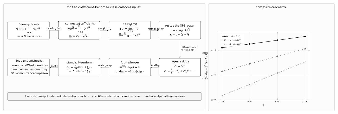
The algebraic lane must be followed in order: form logarithmic connected coefficients before taking $h=b^2\to0$, restore the OPE logarithm, and only then differentiate. The numerical lane integrates the rational oper around $0$ and $t$. Retaining $\kappa/t$, then $f_1$, then $2f_2t$ makes the composite-trace error scale respectively as $t$, $t^2$, and $t^3$.

Direct monodromy integration tests every retained order

For the rational slice, parameterize a counterclockwise circle enclosing $0$ and $t$ but not $1$:

$$z(\phi) = \frac t2 +\frac15\ee^{\ii\phi}, \qquad 0\le\phi\le2\pi.$$

Rewrite the oper as the first-order system

$$\frac{\dd Y}{\dd\phi} = z'(\phi) \begin{pmatrix} 0&1 \\ -T_{\mathrm{op}}(z(\phi);t)&0 \end{pmatrix} Y, \qquad Y(0)=\mathbb I.$$

The target trace is

$$\operatorname{tr}Y(2\pi) = \frac{\sqrt5-1}{2}.$$

The following table uses 40 decimal digits and 5000 fixed fourth-order Runge–Kutta steps. The last column is the maximum, over the three truncations, of the final determinant error at $\phi=2\pi$.

| $t$ | only $\kappa/t$ | through $f_1$ | through $f_2$ | $\max_{\rm trunc.}|\det Y(2\pi)-1|$ | |---:|---:|---:|---:|---:| | $0.08$ | $1.31598\times10^{-1}$ | $1.34068\times10^{-2}$ | $1.18033\times10^{-3}$ | $5.4\times10^{-18}$ | | $0.04$ | $6.47600\times10^{-2}$ | $3.27486\times10^{-3}$ | $1.44123\times10^{-4}$ | $4.6\times10^{-18}$ | | $0.02$ | $3.21239\times10^{-2}$ | $8.09097\times10^{-4}$ | $1.78100\times10^{-5}$ | $4.4\times10^{-18}$ | | $0.01$ | $1.59984\times10^{-2}$ | $2.01072\times10^{-4}$ | $2.21368\times10^{-6}$ | $4.4\times10^{-18}$ |

Each halving of $t$ reduces the three errors by factors approaching $2$, $4$, and $8$. This is the expected order-by-order signature:

$$\begin{aligned} \left| \operatorname{tr}M_{0t} -\frac{\sqrt5-1}{2} \right| &= O(t) && \text{with only }\kappa/t, \\ &= O(t^2) && \text{through }f_1, \\ &= O(t^3) && \text{through }f_2. \end{aligned}$$

The determinant check tests the integrator and the traceless first-order matrix. It does not replace the trace check, which tests the accessory coefficients themselves.

The complete reproducible script is classical-block-monodromy-check.py. It records the parameters, branch, contour, precision, step count, target trace, and both error measures.

Painlevé VI gives a second construction, not an object identity

The same four-puncture monodromy problem can be embedded into a Painlevé VI flow. Branchwise, the classical block can be represented by a regularized on-shell PVI action for a boundary-value problem whose small-$t$ asymptotics encode the internal channel and whose endpoint condition removes an apparent singularity in the desired oper.

This representation is powerful for two reasons:

• the Hamilton–Jacobi derivative reproduces the accessory coefficient;
• the PVI boundary problem supplies an independent recursive route to the small-$t$ accessory series.

It must nevertheless be stated precisely. The holomorphic classical block is not simply $\Log\tau_{\mathrm{JMU}}$. The classical $c_{\mathrm{Vir}}\to\infty$ action, the analytic $c_{\mathrm{Vir}}=1$ tau function, and the full Liouville action are related constructions with different normalizations and boundary data.

For fixed asymptotic monodromy labels, more than one PVI trajectory can satisfy related endpoint conditions. The branch naturally connected to the chosen small-$t$ block is selected by continuation from its sewing germ. Global uniqueness is not implied.

A computation protocol that survives normalization changes

For a generic four-point problem:

1. Declare the ODE convention. Record the puncture order, normal form, loop product, scalar/system lift, and standard-Heun convention.
2. Choose exponent lifts. Compute $\delta_i=(1-\theta_i^2)/4$ and $d=(1-\theta_{0t}^2)/4$ before using any trace periodicity.
3. Fix the block normalization. State whether the OPE power is included. Record the chosen branch of $\Log t$.
4. Generate exact quantum coefficients. Use Gram matrices, Zamolodchikov recursion, or an equivalent finite-$c$ construction.
5. Take the logarithm first. Form the connected coefficients $\ell_N$ before the heavy limit.
6. Extract the classical jet. Evaluate $f_N=\lim_{h\to0}h\ell_N$ and monitor Kac denominators.
7. Restore the channel logarithm. Use $f=\kappa\Log t+\widehat f$.
8. Differentiate at fixed data. Obtain $c_t=\kappa/t+\sum n f_nt^{n-1}$.
9. Convert conventions exactly. Reconstruct $c_0,c_1$ and then apply the affine Heun map; never identify $q_{\mathrm H}$ directly with $\partial_tf$.
10. Use two independent checks. At minimum, combine an annulus or Ward check with direct monodromy, recurrence, or a PVI calculation.
11. Continue only after the germ passes. Record the path and monitor singular divisors or branch exchanges.

Precision planning

At level $N$, the separate quantum coefficient can grow like $h^{-N}$ while the logarithmic remainder grows only like $h^{-1}$. Roughly $(N-1)|\log_{10}h|$ decimal digits can be lost to cancellation before ordinary numerical errors are counted. Exact rational algebra is ideal at low levels. At higher levels, increase the working precision as $h$ decreases and demand a stable extrapolation under both changes.

What this page determines

Output	Determined here?	Additional data
Unit-leading classical block germ	Yes, through the chosen truncation	Channel, lifts, branch, and genericity
Full classical block germ	Yes, after restoring $\kappa\Log t$	Same
Four-pole oper	Yes	Fixed modulus and accessory branch
Standard Heun accessory $q_{\mathrm H}$	Yes	Declared scalar gauge and sign lifts
One composite-monodromy conjugacy class	Yes	Ordered separating loop and lift
Conjugate twist coordinate	Not from $\partial_tf$ alone	A $t$-independent generating-function normalization
Normalized local Frobenius frames	No	Endpoint coordinates and leading coefficients
Connection matrix	No	Fusion/braiding, continuation, and basis normalizations
Full Liouville correlator or uniformizing saddle	No	Spectrum, structure constants, antiholomorphic pairing, and a saddle prescription
Global single-valued branch	No	Analytic continuation and branch selection

Common pitfalls

Taking the heavy limit before the logarithm. Individual $\mathcal V_N$ have stronger divergences than the connected coefficients. Form $\ell_N$ first.

Using the unit-leading derivative as the full accessory. $\partial_t\widehat f$ omits $\kappa/t$ and fails the sewing-annulus check.

Calling the standard Heun parameter the accessory derivative. $c_t^{\mathrm{op}}=\partial_tf$ is a normal-form residue. $q_{\mathrm H}$ is its affine image under a declared scalar gauge.

Reducing the internal exponent modulo the trace too early. The trace forgets the logarithmic lift. Shifted representatives can select different weights and accessory branches.

Substituting a Kac value into a generic rational coefficient. A zero Gram determinant invalidates the inverse-matrix formula. Construct the appropriate quotient or limiting combination first.

Confusing local convergence with global uniqueness. A convergent small-$t$ germ can still meet branch changes under continuation.

Equating fixed composite trace with complete monodromy. The character variety also has a conjugate twist coordinate.

Inferring a connection coefficient from the equation. The oper does not normalize its endpoint bases or choose a continuation path.

Exercises

1. Derive the logarithmic recursion

Starting from

$$\widehat{\mathcal V}(t) = \exp \left( \sum_{n\ge1}\ell_nt^n \right),$$

derive the recursion for $\ell_N$ in terms of the block coefficients $\mathcal V_N$.

Solution

Differentiate and multiply by $t$:

$$t\widehat{\mathcal V}'(t) = \left( \sum_{k\ge1}k\ell_kt^k \right) \widehat{\mathcal V}(t).$$

With $\mathcal V_0=1$, the coefficient of $t^N$ is

$$N\mathcal V_N = \sum_{k=1}^{N} k\ell_k\mathcal V_{N-k}.$$

Isolating the $k=N$ term gives

$$\ell_N = \mathcal V_N -\frac1N \sum_{k=1}^{N-1} k\ell_k\mathcal V_{N-k}.$$

2. Recover the level-one coefficient

Use the level-one Gram matrix and the heavy scaling to derive $f_1$.

Solution

At level one,

$$\mathcal V_1 = \frac{ (\Delta+\Delta_t-\Delta_0) (\Delta+\Delta_1-\Delta_\infty) }{ 2\Delta }.$$

Under $\Delta_j=\delta_j/h+O(1)$,

$$\mathcal V_1 = \frac1h \frac{ (d+\delta_t-\delta_0) (d+\delta_1-\delta_\infty) }{ 2d } +O(1).$$

Multiplying by $h$ gives

$$f_1 = \frac{AB}{2d}.$$

3. Locate the first two inverse-Gram singularities

Translate $d=0$ and $4d+3=0$ into the internal exponent $\theta_{0t}$.

Solution

Since

$$d = \frac{1-\theta_{0t}^2}{4},$$

$d=0$ gives $\theta_{0t}^2=1$. Moreover,

$$4d+3 = 1-\theta_{0t}^2+3 = 4-\theta_{0t}^2,$$

so $4d+3=0$ gives $\theta_{0t}^2=4$. These are singularities of the generic level-one and level-two inverse-Gram expressions, respectively.

4. Complete the rational level-two arithmetic

For the rational slice on this page, verify $f_2=587/11700$.

Solution

For pairwise equal external weights, $A=B=d$ and

$$P=d+\delta_t, \qquad Q=d+\delta_1.$$

Substitution into the general result simplifies it to

$$f_2 = \frac{ 13d^2 +4d\delta_t +4d\delta_1 +9d +16\delta_t\delta_1 }{ 16(4d+3) }.$$

Using

$$d=\frac4{25}, \qquad \delta_t=\frac29, \qquad \delta_1=\frac6{25}$$

and reducing the rational number gives

$$f_2 = \frac{587}{11700}.$$

5. Check both Ward constraints

Starting from the displayed $c_t$, derive $c_0$ and $c_1$ through the shown orders and verify the two relations at infinity.

Solution

Use

$$c_0=-\Lambda+(t-1)c_t, \qquad c_1=\Lambda-tc_t.$$

With

$$c_t = -\frac{64}{225t} +\frac2{25} +\frac{587}{5850}t +O(t^2)$$

and $\Lambda=-4/9$,

$$\begin{aligned} c_0 &= \frac{64}{225t} +\frac2{25} -\frac{119}{5850}t +O(t^2), \\ c_1 &= -\frac4{25} -\frac2{25}t -\frac{587}{5850}t^2 +O(t^3). \end{aligned}$$

Direct addition gives $c_0+c_t+c_1=0$ through the retained order. Substitution into

$$\delta_0+\delta_t+\delta_1+tc_t+c_1$$

leaves $\delta_\infty=6/25$.

6. Derive the Heun coefficient recursion

Show that for $n\ge2$,

$$[t^n]\,q_{\mathrm H} = n f_n-(n-1)f_{n-1}.$$

Solution

Only the first two terms of

$$\frac{\gamma_{\mathrm H}}2 (t\delta_{\mathrm H}+\epsilon_{\mathrm H}) +t\Lambda$$

contribute at degrees zero and one. For the remaining factor,

$$\begin{aligned} -t(t-1)c_t &= t(1-t) \left[ \frac{\kappa}{t} +\sum_{m\ge1}m f_mt^{m-1} \right] \\ &= \kappa(1-t) +\sum_{m\ge1} m f_m \left( t^m-t^{m+1} \right). \end{aligned}$$

At degree $n\ge2$, the coefficient is therefore $n f_n-(n-1)f_{n-1}$.

7. Match the two monodromy lifts

For $\theta_{0t}=3/5$, find a representative $\sigma_{0t}$ in the traceless-system convention and verify the two traces exactly.

Solution

Choose

$$\sigma_{0t} = 1-\theta_{0t} = \frac25.$$

Then

$$\begin{aligned} -2\cos(\pi\theta_{0t}) &= -2\cos\frac{3\pi}{5} \\ &= \frac{\sqrt5-1}{2} \\ &= 2\cos\frac{2\pi}{5} \\ &= 2\cos(\pi\sigma_{0t}). \end{aligned}$$

8. Reproduce the monodromy-order test

Run the linked script at 40 digits with 5000 and 10,000 steps. Estimate the convergence order under $t\mapsto t/2$ for all three accessory truncations, and check that the reported trace errors are stable while the determinant errors decrease.

Solution

For successive errors $E(t)$ and $E(t/2)$, estimate

$$p(t) = \frac{ \Log[E(t)/E(t/2)] }{ \Log2 }.$$

The estimates approach $1$, $2$, and $3$ for the three truncations. Doubling the step count changes the trace errors far below their displayed digits. For this final-determinant diagnostic, the error decreases by approximately $2^5$; that superconvergent scalar check should not be used to infer the global order of the matrix solution. Record the software version, precision, contour radius, step count, and target trace with the output.

References

• M. Beşken, S. Datta, and P. Kraus, “Semi-Classical Virasoro Blocks: Proof of Exponentiation”, Journal of High Energy Physics 2020 (1), 109. Section 3 proves generic four-point exponentiation in the oscillator formulation; Appendix A treats the generic linear-system nondegeneracy.
• M. Gerbershagen and J. Hollweck, “Exponentiation of Higher-Point and Higher-Genus Virasoro Conformal Blocks in the Semiclassical Limit”, arXiv:2606.18345. Explicitly formulates semiclassical exponentiation at the level of a formal power series and extends the oscillator argument beyond the four-point sphere.
• A. Litvinov, S. Lukyanov, N. Nekrasov, and A. Zamolodchikov, “Classical Conformal Blocks and Painlevé VI”, Journal of High Energy Physics 2014 (7), 144. Equations (1.5)–(1.8) state the classical scaling and sewing normalization; equations (2.7)–(2.17) derive the BPZ oper, accessory gradient, and composite trace; Section 3 gives the regularized PVI action.
• J. Teschner, “Classical Conformal Blocks and Isomonodromic Deformations”, arXiv:1707.07968. Equations (3.13)–(3.17) identify the classical generating function and its oper and monodromy derivatives; Section 4 distinguishes a holomorphic block from the uniformizing Liouville saddle.
• M. Lencsés and F. Novaes, “Classical Conformal Blocks and Accessory Parameters from Isomonodromic Deformations”, Journal of High Energy Physics 2018 (4), 096. Equations (1.3)–(1.4), Section 4, and Appendix C give the sign bridge, isomonodromic construction, and accessory expansion.
• M. Piątek and A. R. Pietrykowski, “Solving Heun’s Equation Using Conformal Blocks”, Nuclear Physics B 938 (2019), 543–570. Proposition 1.1 and equation (2.13) relate the classical derivative to path-multiplicative Heun solutions and the scalar composite trace.
• P. Menotti, “Convergence of Classical Conformal Blocks”, Journal of Physics A: Mathematical and Theoretical (2026). Gives an all-orders algebraic recursion and proves a nonzero local convergence radius under nondegeneracy assumptions.
• A. B. Zamolodchikov, “Conformal Symmetry in Two Dimensions: An Explicit Recurrence Formula for the Conformal Partial Wave Amplitude”, Communications in Mathematical Physics 96 (1984), 419–422. Gives the earlier finite-central-charge recurrence for conformal partial waves.
• A. B. Zamolodchikov, “Conformal Symmetry in Two-Dimensional Space: Recursion Representation of Conformal Block”, Theoretical and Mathematical Physics 73 (1987), 1088–1093. Introduces the elliptic uniformizing-variable recurrence used for high-level block computation.
• NIST Digital Library of Mathematical Functions, §31.2, “Differential Equations”, especially equations (31.2.1)–(31.2.3) for the standard and normal Heun forms.