Appendix C: Computational Laboratory

A numerical value is reproducible only when three layers are recorded separately: the exact mathematical object, the finite algorithm used to approximate it, and the evidence supporting the reported digits. Increasing precision controls only part of the third layer. It cannot repair a wrong branch, a reversed connection matrix, an open lift mistaken for a cycle, or a discretized equation that differs from the intended continuum problem.

This appendix is a cross-method bench manual. It gives a common protocol for the book’s local-series, recurrence, monodromy, period, Borel–Padé, and TBA calculations, then links to the pages and programs where each method is developed in depth.

The laboratory contract

Freeze the mathematical passport before choosing an algorithm. Vary one numerical control at a time. Preserve raw refinement data. Compare invariants before comparing decimal strings. Call a result certified only when outward-rounded enclosures and an applicable theorem prove the declared claim.

A frozen passport precedes every calculation

Let $F$ be an exact scalar characteristic function, period, matrix entry, or nonlinear residual. Let $F_N$ be a finite approximation and $\widehat F_{N,p}$ its evaluation at working precision $p$. At a computed candidate $\widehat\lambda$,

$$\begin{aligned} F(\widehat\lambda) ={}& \bigl[F-F_N\bigr](\widehat\lambda) \\ &+ \bigl[F_N-\widehat F_{N,p}\bigr](\widehat\lambda) \\ &+ \widehat F_{N,p}(\widehat\lambda). \end{aligned}$$

The three rows are truncation or discretization error, arithmetic evaluation error, and nonlinear-solve residual. Conditioning is needed to turn their sum into an error in $\lambda$. A model or dictionary error is more basic: it changes $F$ itself and therefore does not belong in this additive budget.

The book uses the following evidence labels.

Label	Minimum support
Computed	One declared finite algorithm returns a candidate
Internally converged	Independent controls such as cutoff, order, mesh, contour panels, and precision have stable refinement tables
Cross-verified	A representation with substantially different failure modes agrees under its own refinements
Certified	Outward-rounded bounds plus an inclusion, root-count, or uniqueness theorem prove the stated conclusion

Physical or interpretive validation is an orthogonal question. A certified root of the wrong boundary problem remains the wrong observable.

Every method card should freeze five groups of data.

Group	Required data
Object	Equation, exact parameters, gauge, normalization, boundary or connection datum
Analytic	Branches, cuts, path or contour, sheet, cycle, chamber, and lateral side
Finite model	Series order, recurrence depth, Padé shape, grid, panels, cutoff, and tail model
Arithmetic	Input provenance, working precision, guard digits, rounding, solver, and stopping norm
Evidence	Invariants, refinement table, conditioning estimate, independent representation, and claim label

A useful planning estimate is

$$d_{\mathrm{work}} \gtrsim d_{\mathrm{goal}} + \left\lceil \log_{10}\kappa_{\mathrm{cond}} \right\rceil +g,$$

where $\kappa_{\mathrm{cond}}\geq1$ estimates lost digits and $g$ is a guard margin. This is a budget, not a validation theorem.

Pathwise transport preserves an ordered frame

Write a linear ODE as

$$\frac{\dd Y}{\dd z} = A(z,\lambda)Y.$$

Along a declared path $z=\gamma(t)$, $0\leq t\leq1$, integrate

$$\frac{\dd Y}{\dd t} = \gamma'(t) A(\gamma(t),\lambda)Y.$$

The path parameterization, initial ordered frame, and every rescaling belong to the result. A robust high-precision transport proceeds as follows.

1. Seed a normalized local jet inside a certified or well-tested convergence disk, rather than directly at a singular point.
2. Split the path before coefficient singularities, sharp bends, or regions where exponential separation exhausts the guard digits.
3. Refine step size, method order, and precision independently. A last-term or step-doubling estimate is evidence unless a remainder theorem has been supplied.
4. Rescale columns or use QR factorizations when necessary, but preserve the noncommuting factor order. If $Y=QH$ and a transport step gives $\widetilde Q=Q_{\mathrm{new}}R$, update $H_{\mathrm{new}}=RH$: each new factor multiplies the accumulator on the left.
5. Evaluate an off-mesh ODE residual and repeat the transport in reverse.

Arbitrary precision reduces roundoff; it does not validate the IVP solver. If a Taylor step is analytic on $|s|\leq r$, a Cauchy bound can convert the local truncation into a proof. Without such a bound, order and step ladders remain convergence evidence.

Liouville’s formula supplies a cheap invariant. For transport from $t=0$ to $t=1$,

$$\frac{ \det Y(1) }{ \det Y(0) } = \exp\left[ \int_\gamma \operatorname{tr}A(z,\lambda)\,\dd z \right].$$

It detects many frame and integration failures, although a correct determinant does not determine the individual matrix entries.

Monodromy is endpoint transport around a loop

For a based loop and an initial frame $B=Y(0)$, the house right action gives

$$Y(1)=B M_\gamma, \qquad M_\gamma=B^{-1}Y(1).$$

Numerically solve the linear system rather than forming $B^{-1}$. If $B=I$, the final transported frame is the monodromy matrix. The path product $\gamma_1\gamma_2$ traverses $\gamma_2$ first and then $\gamma_1$, so

$$M_{\gamma_1\gamma_2} = M_{\gamma_1}M_{\gamma_2}.$$

Path ordering cannot be replaced by $\exp\!\int_\gamma A\,\dd z$ unless the coefficient matrices commute along the path. Audit a loop computation by checking

$$M_{\gamma^{-1}}M_\gamma\approx I,$$

Liouville’s determinant, local nonresonant eigenvalues $\ee^{2\pi\ii\rho_j}$, the declared generator product, homotopic loop deformations, and simultaneous conjugation under a common frame change. Near a Jordan block, traces and determinants are much more stable than eigenvectors.

The global-data chapter fixes the path and matrix conventions. Its hypergeometric benchmark provides exact monodromy data against which a transport code can be calibrated.

Overlapping series turn local data into connection matrices

At a regular singular point, a normalized Frobenius branch has the form

$$y(z) = (z-z_0)^\rho \sum_{n\geq0}c_n(z-z_0)^n.$$

Record the local coordinate, exponent lift, branch of $\operatorname{Log}(z-z_0)$, leading coefficient, recurrence, and analytic disk. Evaluate $y$ and $y'$ from the same coefficient list. A proved ratio bound

$$\left| \frac{ c_{n+1}\delta^{n+1} }{ c_n\delta^n } \right| \leq q<1, \qquad n\geq N+1,$$

gives the value-tail enclosure

$$\left| \sum_{n>N}c_n\delta^n \right| \leq \frac{ |c_{N+1}\delta^{N+1}| }{ 1-q }.$$

This bounds the analytic factor $\sum c_n\delta^n$. The full solution-tail bound carries the declared-branch multiplier $|\delta^\rho|$. The derivative needs its own bound with $|\delta^{\rho-1}|$ and the additional $|n+\rho|$ factor.

Continue through overlapping Frobenius or ordinary Taylor disks, keeping each new center strictly inside the preceding analytic disk. In a common overlap the house direction is

$$\Phi_\beta = \Phi_\alpha C_{\alpha\beta}, \qquad C_{\alpha\beta} = \Phi_\alpha(z_m)^{-1}\Phi_\beta(z_m).$$

Again, solve for $C_{\alpha\beta}$ rather than explicitly inverting a poorly conditioned frame. Move $z_m$ through the overlap, reverse the match, verify the Abel determinant, and compare with pathwise ODE transport. A drift with $z_m$ measures numerical error; it is not new connection data.

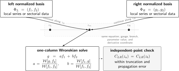
Local bases become global connection data only after their gauges, branches, derivative coordinate, and continuation paths agree. An independent match point tests every matrix entry, whereas the determinant supplies only one necessary invariant.

When exponent differences are integral, use a logarithmic Frobenius basis or a controlled resonant limit. Evaluating a nearly singular generic basis at more digits can still be far less stable than changing the basis first. The Frobenius and Leaver page derives the local recurrences, and the connection-matrix page develops the matching invariants.

Minimal recurrences impose a boundary condition at infinity

For a three-term recurrence

$$\alpha_nu_{n+1} + \beta_nu_n + \gamma_nu_{n-1} =0,$$

define

$$R_n := \frac{u_n}{u_{n-1}}.$$

The backward Riccati map is

$$R_n = -\frac{ \gamma_n }{ \beta_n+\alpha_nR_{n+1} }.$$

First establish the minimal-solution or continued-fraction theorem in the parameter domain of interest. Then seed a terminal approximation $R_{N+1}^{(K)}$ from $K$ large-order terms and sweep backward. A projective pair $R_{n+1}=p/q$ updates homogeneously as

$$(p,q) \longmapsto \left( -\gamma_nq, \beta_nq+\alpha_np \right),$$

with rescaling after every step. This chart survives values for which a scalar ratio overflows.

If the endpoint row is

$$\alpha_0u_1+\beta_0u_0=0,$$

the minimal-line residual is

$$F(\lambda) = \beta_0(\lambda) + \alpha_0(\lambda)R_1^{\min}(\lambda).$$

Vary recurrence depth $N$, tail order $K$, working precision $p$, terminal line, and any split index independently. Differentiate the terminal seed and every coefficient-dependent backward map when computing $F'$. Track ratio poles together with zeros: a pole of one projective chart need not be a spectral singularity.

A backward sweep and a Lentz evaluation mainly test arithmetic. A recurrence root and a direct ODE Wronskian have more independent failure modes. A finite depth becomes certified only after a tail enclosure has been propagated through the Möbius maps and a root-inclusion theorem has been applied. See the minimal-solution page, the continued-fraction page, and the large-order tail page.

Period quadrature must remain on the spectral cover

For

$$\widehat\Sigma: \qquad y^2=Q(z), \qquad \lambda=y\,\dd z,$$

a projected contour is not enough. Store its orientation, initial sheet, cut crossings, lifted endpoints, and deleted poles. Along projected nodes $z_j$, continue $y$ analytically; do not call an independent principal square root at each node. Away from turning points, a useful predictor is

$$y_{j+1}^{\mathrm{pred}} = y_j + \frac{Q'(z_j)}{2y_j} (z_{j+1}-z_j),$$

after which the sign of $\sqrt{Q(z_{j+1})}$ closest to the predictor is chosen. This still requires step refinement and fails if used coarsely near $y=0$.

At a simple branch point $a$, set

$$z-a=t^2.$$

Since $Q(z)=Q'(a)(z-a)+O((z-a)^2)$,

$$y\,\dd z \sim 2\sqrt{Q'(a)}\,t^2\,\dd t,$$

so the lifted integrand is regular in $t$. For a cut cycle whose chosen bank runs from $a$ to $b$,

$$\oint_\gamma\lambda = 2\int_a^b y_+(z)\,\dd z,$$

with the sign fixed by the sheet and orientation.

A numerical closed lift must return to the same $z$ and the same sheet. Audit path reversal, the deck involution, homology relations, contour deformation away from poles, residue jumps when a pole is crossed, and a known Weber or Mathieu closed period. An Airy calibration is instead a normalized relative action. Refine branch-point locations, panels, quadrature order, and precision separately. Picard–Fuchs or Gauss–Manin continuation is a valuable independent representation when available.

The spectral-cover page fixes the geometry, while the cycle and residue page and the regularized-period page explain which lifted forms may actually be integrated at each WKB order.

Borel–Padé separates continuation from quadrature

For the shifted house convention,

$$\mathcal B\widehat f(\xi) = \sum_{k\geq0} b_k\xi^k, \qquad b_k=\frac{a_{k+1}}{k!}.$$

From $K$ available coefficients construct a near-diagonal rational function

$$R_{L,M}(\xi) = \frac{P_L(\xi)}{Q_M(\xi)}, \qquad Q_M(0)=1, \qquad L+M+1\leq K.$$

Use exact or guard-precision linear algebra, verify the matched Taylor coefficients, and inspect a triangle of nearby $(L,M)$ values. Stable poles, zeros, and residues are more informative than a single plot. A moving close pole–zero pair is often a Froissart defect; an alternating stable chain may represent a cut and must not be deleted automatically.

Before calling the result a Borel sum, verify analytic admissibility of the continued transform. If, for some $C>0$ and $\sigma\geq0$,

$$\left| \mathcal B\widehat f(\ee^{\ii\theta}t) \right| \leq C\ee^{\sigma t},$$

then the actual Laplace integral requires

$$\operatorname{Re} \left( \frac{\ee^{\ii\theta}}{\hbar} \right) > \sigma.$$

For the finite rational surrogate, a pole-free prescribed contour and the weaker condition with right-hand side zero suffice. Convergence of that surrogate integral alone does not prove that the original formal series is Borel summable in the direction.

For a declared ray and lateral side, evaluate

$$\mathcal S_\theta^{[L/M]}\widehat f = a_0 + \ee^{\ii\theta} \int_0^\infty \ee^{-\ee^{\ii\theta}t/\hbar} R_{L,M}(\ee^{\ii\theta}t) \,\dd t.$$

Record contour splits, pole clearance, quadrature rule, finite Laplace cutoff, and rational tail bound. Those bounds validate the integral of the chosen rational surrogate; they do not supply a generic bound on the unknown Padé continuation error. Separate coefficient, Padé-shape, contour, quadrature, and tail refinements.

The mandatory normalization tests are a monomial and the factorial one-pole model from Appendix B. The full Borel–Padé laboratory adds withheld-coefficient tests, lateral signs, root counts, and independent spectral determinants.

TBA residuals and continuum errors are different

Write a nonlinear integral equation schematically as

$$\varepsilon = \mathcal T(\varepsilon) = d+S+\mathcal K L(\varepsilon), \qquad L(z)=\operatorname{Log}(1+\ee^{-z}).$$

Freeze the logarithm sheet, integration contour and banks, source divisor, chamber, asymptotic subtraction, and observable before discretizing. Use Nyström panels on general contours. Use an FFT only when translation invariance justifies convolution, and zero-pad to the linear-convolution length rather than silently periodizing the line. Retain every quadrature weight and state whether $1/(2\pi)$ is part of the kernel.

Let $\mathcal R_N$ restrict a function to the grid, let $\mathcal I_N$ reconstruct a function from grid data, and let $\widehat\varepsilon_N$ be the computed grid vector. Set

$$\widehat\varepsilon := \mathcal I_N\widehat\varepsilon_N, \qquad \widetilde{\mathcal T}_N := \mathcal I_N\mathcal T_N\mathcal R_N.$$

Now both residuals live in the declared function space. Separate

$$\eta := \left\| \widehat\varepsilon -\widetilde{\mathcal T}_N(\widehat\varepsilon) \right\|$$

from the continuum defect

$$\delta := \left\| \widetilde{\mathcal T}_N(\widehat\varepsilon) - \mathcal T(\widehat\varepsilon) \right\|.$$

If a complete declared set $U$ contains $\widehat\varepsilon$, $\mathcal T(U)\subseteq U$, and $\mathcal T$ is a contraction on $U$ with constant $q<1$, then

$$\left\| \widehat\varepsilon-\varepsilon^* \right\| \leq \frac{\eta+\delta}{1-q}.$$

A small discrete residual alone says nothing about cutoff, quadrature, FFT wrap, or logarithm-sheet error. Damping, Anderson acceleration, and Newton–Krylov methods may improve convergence but do not replace the invariant-set and contraction proof. Excited roots and divisor crossings belong to the nonlinear unknown rather than to post-processing.

Refine the left and right cutoffs, mesh, FFT padding or panel order, precision, nonlinear tolerance, bank offset, continuation step, and root tolerance independently. Compare dense and FFT multiplication on a smaller grid and evaluate an off-grid continuum residual. The TBA numerical laboratory derives these estimates and treats hard branches and excited roots.

Enclosures become conclusions only through a theorem

Ball arithmetic represents a set, for example $x\in[m\mathbin{\pm}r]$, using outward-rounded operations. A narrow output ball encloses the desired exact value only if exact inputs, truncation tails, quadrature remainders, and every intervening operation have also been enclosed.

For a realified nonlinear system $F:\mathbb R^n\to\mathbb R^n$, suppose that $X$ is a box, $x_0\in X$, $C$ is nonsingular, and $F\in C^1$ on a neighborhood of $X$. Let the interval matrix $F'(X)$ enclose every Jacobian $F'(x)$ for $x\in X$. The Krawczyk operator is

$$\begin{aligned} K(X) ={}& x_0-CF(x_0) \\ &+ \left( I-CF'(X) \right) (X-x_0). \end{aligned}$$

If the strict inclusion

$$K(X) \subset \operatorname{int}X$$

holds, then these hypotheses certify a unique zero in $X$. Merely obtaining $0\in F(X)$ is not enough. For analytic scalar functions, Rouché or an argument-principle enclosure can certify a root count instead. The verified-numerics page develops tail balls, conditioning, Rouché, Krawczyk, and the distinction between backward and forward error.

A reproduction record should run without guesswork

Archive the following fields with every publishable result.

Group	Record
Mathematical object	Equation or operator, exact parameters, gauge, normalization, domain, and boundary data
Analytic choices	Branches, cuts, path or contour, sheet, cycle, chamber, and lateral side
Discretization	Orders, cutoffs, grids, panels, seeds, match or split points, and omitted-tail model
Arithmetic	Exact input strings, precision, guard digits, rounding mode, and coefficient provenance
Solve	Initial data, algorithm, tolerance norm, residual scale, derivatives, and conditioning estimate
Audits	Raw refinement table, invariant checks, unused coefficients, and independent representation
Environment	Code revision, exact command, interpreter, libraries, operating system, deterministic seeds, and thread count
Output	Raw data, checksums, reported digits, limitations, and evidence label

Parse non-integer decimal inputs from exact strings. Promoting a binary64 number to a large multiple-precision container does not restore the digits already rounded away. Checks should raise explicit exceptions rather than language assertions that may disappear under optimized execution.

A quick connection-matrix micro-lab

The tested baseline is CPython 3.10 or later with mpmath==1.3.0; this checker requires no other third-party package. From the repository root, run

python3 public/code/advanced-ode/general-heun-connection-check.py \
  --t 0.04 --order 2 --terms 80 --dps 40 \
  --no-table --check-second-point

Then repeat with --terms 160 --dps 80. In the baseline environment, the match-point drift falls from about $2.8800350152674\times10^{-15}$ to $1.8752301676036\times10^{-29}$, while the Abel and direct determinants agree at about $-1.03319670758600654$. The fixed order-two block approximation has a separate model error of about $1.0870188841823\times10^{-5}$ and therefore does not improve with the series cutoff. The experiment distinguishes a converging matching error from a deliberately frozen analytic truncation.

The repository contains a compact smoke suite.

Workflow	Downloadable checker	Principal audit
Frobenius matching	general-heun-connection-check.py	Two match points and Abel determinant
Loop monodromy	classical-block-monodromy-check.py	Composite-loop trace and determinant at one declared step count; rerun with doubled --steps for refinement
Minimal recurrence and exact Bessel bracket	verified-numerics.py	Cutoff–tail–precision tensor and exact Bessel bracket
Lifted WKB actions	wkb-homology-action-check.py	Sheet sign, doubled lift, residues, and Gauss–Manin identity
Borel–Padé and spectra	borel-pade-spectral-check.py	Padé shapes, lateral jump, determinant, and root count
TBA iteration	tba-iteration-check.py	Dense-versus-FFT convolution and cutoff–mesh refinement

Their source docstrings and linked pages state scope and limitations. Passing all of them validates the implementations on their declared benchmarks; it does not prove a new problem that merely resembles those benchmarks.

Common pitfalls

Equating more digits with more evidence. Higher precision can reveal a truncation plateau, but it cannot bound an unproved tail or correct a wrong sheet. Refine the finite model and arithmetic independently.

Forming a matrix inverse because the formula contains one. Solve the linear system and monitor conditioning. Explicit inversion adds avoidable roundoff and hides which frame is ill-conditioned.

Recomputing principal square roots on a lifted contour. This can switch sheets without warning or fail to close a cycle. Continue the initial sheet and refine near every turning point.

Treating a discrete residual as a continuum residual. A nonlinear solver can solve the wrong finite grid to machine precision. Cutoff, quadrature, tail, and aliasing defects require separate estimates.

Calling two codes independent when they share the derivation. Rewriting the same recurrence in another language mainly tests transcription and arithmetic. Compare representations chosen for different failure modes.

Exercises

1. Transport a logarithmic frame

For

$$y''+\frac1z y'=0,$$

use the ordered basis $(1,\operatorname{Log}z)$ and a positive loop around zero. Determine the right-acting monodromy matrix, its determinant, and the matrix for the reverse loop.

Solution

The constant solution returns to itself, while

$$\operatorname{Log}z \longmapsto \operatorname{Log}z+2\pi\ii.$$

Therefore

$$M_0 = \begin{pmatrix} 1&2\pi\ii\\ 0&1 \end{pmatrix}.$$

Its determinant is one. This also follows from Liouville’s formula because $\operatorname{tr}A=-1/z$ in the companion system and

$$\exp\left(-\oint\frac{\dd z}{z}\right) = \ee^{-2\pi\ii} =1.$$

The reverse loop gives

$$M_0^{-1} = \begin{pmatrix} 1&-2\pi\ii\\ 0&1 \end{pmatrix}.$$

A numerical transport should recover both loop matrices and make $\|\widehat M_{\gamma^{-1}}\widehat M_\gamma-I\|$ decrease under step and precision refinement.

2. Recover a minimal line backward

Consider

$$u_{n+1}-3u_n+2u_{n-1}=0.$$

Starting from $R_{N+1}=0$, apply the backward ratio map to obtain $R_1$. Show explicitly that it converges to the minimal ratio.

Solution

The characteristic roots are $1$ and $2$, so the minimal solution is proportional to $1^n$ and has ratio one. Here

$$R_n = \frac{2}{3-R_{n+1}}.$$

After $m$ backward steps from zero,

$$R = \frac{2^{m+1}-2}{2^{m+1}-1}.$$

This follows by induction. Taking $m=N$ gives

$$R_1 = 1- \frac{1}{2^{N+1}-1} \longrightarrow1.$$

Forward recurrence would amplify any contamination by the dominant $2^n$ solution; the backward map selects the minimal line.

3. Smooth a branch-point panel

Let $y^2=z^2-a^2$ with $a>0$. On the bank above $[-a,a]$, choose $y=+\ii\sqrt{a^2-x^2}$ and orient the bank from $-a$ to $a$. Use $x=a\sin t$ to evaluate the doubled cut-cycle period and explain why the endpoint quadrature is regular.

Solution

For $-\pi/2\leq t\leq\pi/2$,

$$x=a\sin t, \qquad y=\ii a\cos t, \qquad \dd x=a\cos t\,\dd t.$$

Thus the lifted integrand is the smooth function $\ii a^2\cos^2t\,\dd t$. The one-bank action is

$$\int_{-a}^{a}y\,\dd x = \ii a^2 \int_{-\pi/2}^{\pi/2} \cos^2t\,\dd t = \frac{\ii\pi a^2}{2}.$$

The oppositely oriented return on the other sheet contributes the same value, so

$$\oint_\gamma y\,\dd z = \ii\pi a^2.$$

Reversing the cycle or the initial sheet reverses the sign.

4. Convert a fixed-point residual into an error bound

Let $U$ be a complete invariant set, let $\mathcal T:U\to U$ be a contraction with constant $q<1$, and let $\widetilde{\mathcal T}_N$ be a reconstructed discrete operator on the same function space. Suppose $\widehat\varepsilon\in U$ and $\|\widehat\varepsilon- \widetilde{\mathcal T}_N(\widehat\varepsilon)\|\leq\eta$ and $\|\widetilde{\mathcal T}_N(\widehat\varepsilon) -\mathcal T(\widehat\varepsilon)\|\leq\delta$. Prove the bound used in the TBA section.

Solution

Let $\varepsilon^*=\mathcal T(\varepsilon^*)$. Then

$$\begin{aligned} \|\widehat\varepsilon-\varepsilon^*\| \leq{}& \|\widehat\varepsilon -\mathcal T(\widehat\varepsilon)\| \\ &+ \|\mathcal T(\widehat\varepsilon) -\mathcal T(\varepsilon^*)\|. \end{aligned}$$

The first term is at most $\eta+\delta$ and the second at most $q\|\widehat\varepsilon-\varepsilon^*\|$. Moving it to the left gives

$$\|\widehat\varepsilon-\varepsilon^*\| \leq \frac{\eta+\delta}{1-q}.$$

Without a proved invariant set and contraction constant, the same algebra is only a heuristic conditioning estimate.

5. Classify a high-precision spectral claim

A program prints 60 stable digits of a recurrence root when the working precision is raised from 100 to 200 digits. It reports one depth $N$, gives no tail remainder, uses no second representation, and archives neither branch data nor the command. Classify the claim and list the next controls needed before it can be called internally converged, cross-verified, or certified.

Solution

The result is computed with a precision refinement. It is not yet internally converged because recurrence depth, tail order, terminal line, split chart, and root-solver tolerance were not varied, and the analytic branch was not recorded.

Internal convergence requires those independent ladders, retained and first omitted recurrence residuals, conditioning information, and a complete passport. Cross-verification additionally requires a representation with different failure modes, such as endpoint-adapted ODE integration and an Abel-normalized Wronskian. Certification further requires outward-rounded coefficient and tail enclosures propagated to a Rouché, Krawczyk, or equivalent inclusion theorem. The exact command, code revision, dependency versions, inputs, and raw tables must be archived at every level.

References

• NIST DLMF, §2.7 Differential Equations, §3.6 Linear Difference Equations, §3.7 Ordinary Differential Equations, §3.10 Continued Fractions, and §31.18 Methods of Computation, for the standard analytic and numerical reference formulae.
• À. Jorba and M. Zou, “A Software Package for the Numerical Integration of ODEs by Means of High-Order Taylor Methods”, Experimental Mathematics 14 (2005), 99–117.
• M. Mezzarobba, “NumGfun: a Package for Numerical and Analytic Computation with D-finite Functions”, ISSAC 2010, 139–145, and “Rigorous Multiple-Precision Evaluation of D-finite Functions in SageMath”, for pathwise series continuation and rigorous evaluation.
• W. Gautschi, “Computational Aspects of Three-Term Recurrence Relations”, SIAM Review 9 (1967), 24–82.
• P. Molin and C. Neurohr, “Computing Period Matrices and the Abel–Jacobi Map of Superelliptic Curves”, Mathematics of Computation 88 (2019), 847–888.
• G. A. Baker Jr. and P. Graves-Morris, Padé Approximants, second edition, Cambridge University Press (1996).
• P. Dorey and R. Tateo, “Anharmonic Oscillators, the Thermodynamic Bethe Ansatz, and Nonlinear Integral Equations”, Journal of Physics A 32 (1999), L419–L425.
• S. M. Rump, “Verification Methods: Rigorous Results Using Floating-Point Arithmetic”, Acta Numerica 19 (2010), 287–449.
• F. Johansson, “Arb: Efficient Arbitrary-Precision Midpoint-Radius Interval Arithmetic”, IEEE Transactions on Computers 66 (2017), 1281–1292, and “Numerical Integration in Arbitrary-Precision Ball Arithmetic”, ICMS 2018, 255–263.
• G. K. Sandve et al., “Ten Simple Rules for Reproducible Computational Research”, PLoS Computational Biology 9 (2013), e1003285.